


Selection on observables, covariate-specific trends and conditional parallel trends with difference-in-differences: Pedro's Checklist, Step 4(d)
Selection on observables, covariate-specific trends and conditional parallel trends with difference-in-differences: Pedro's Checklist, Step 4(d)

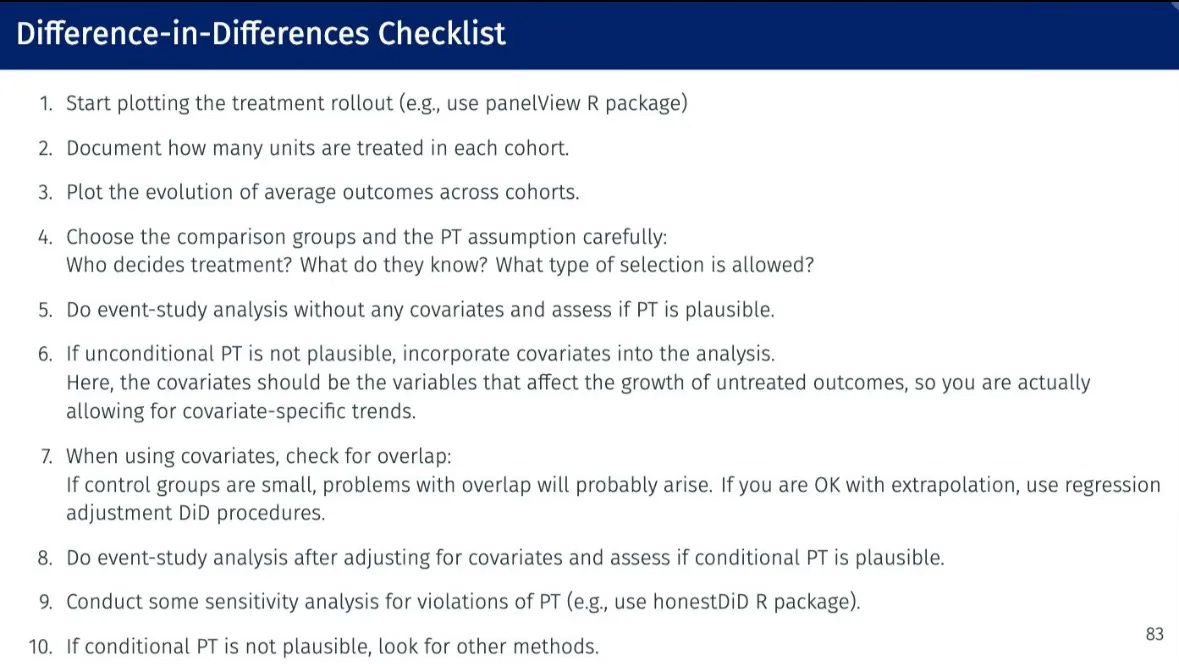
When everyone was first hearing about the “standard” twoway fixed effects specification being biased in differential timing scenarios, it was not uncommon to hear or read authors say something to the effect that since they didn’t have differential timing, they were going to use twoway fixed effects, and then commence to include a variety of covariates. Today I will do a short substack illustrating the bias of two way fixed effects when you have covariate specific parallel trends with other forms of covariate-based heterogeneity. This is part my longer series on “Pedro’s Checklist”, a nice checklist that Pedro Sant’Anna created to guide researchers through choices made when estimating causal effects with difference-in-differences.
Selection on observables and conditional parallel trends
There will be a simulation for this as I wanted to both show you the “ground truth” (i.e., the true causal effect) as well as show you some syntax. I’m going to introduce two things in this data generating process. The first is that I am going to have it where units select into the treatment based on their observable covariates. In my case it will be based on their age and high school GPA in a study about the returns to college on earnings. In this sense, I am wanting to continue to explore the various selection processes that Ghanem, et al. (2024) outline to describe what will or will not “kill” parallel trends.
But the second part of this data generating process will be that parallel trends only holds conditional on covariates. What does this mean. Consider the idea that parallel trends holds but you have different compositions of people in the treatment and control group. Perhaps the treatment group consists of cities, for instance, but the control group consists of suburbs or rural areas. Maybe you’re wanting to know the effect of building a large stadium in the cities on tax revenue. Parallel trends means that the urban cities that built a stadium would have evolved similar to that of the rural and suburban areas had the stadium never been built.
When you doubt that your treatment and control group would have had similar counterfactual trends because of the very different distribution of covariates within treatment and within control, then you are doubting your parallel trends assumption. But if you believe that parallel trends holds similar for treatment and control once you condition on population size, then you are saying parallel trends does hold — it just holds for the high population areas in one way, and the low population areas in another way.
This is what is meant by “conditional parallel trends” and the first time I ever saw the equation for it was in Heckman, Ichimura and Todd (1997) (an unnumbered equation between equations A-4’ and A-5 on page 613). It is also the assumption in Abadie (2005) as well as more recently Sant’Anna and Zhou (2020).
Conditional parallel trends is actually not usually what people, though, have in mind when they are estimating regression models with covariates. They usually have in mind omitted variable bias, or unconfoundedness. But when you are estimating models with difference-in-differences, you are explicitly appealing to parallel trends which already assumes there are no confounders. You are saying in other words that the mean potential outcome, Y(0), would have evolved the same for the two groups, so if they are evolving the same for the two groups, what then do we say about the confounders? They either must not exist, must not matter, or are the same for both treatment and control.
Conditional parallel trends is not an appeal to unconfoundedness, in other words. It is rather simply an appeal to the idea that different units have different trends based on their covariates, but that units with similar covariates have similar counterfactual trends, and that’s it. So then what is it that is generating my conditional parallel trends?
First, I have selection on observables. Units with higher GPA and older ages are more likely to be in the treatment group than the control group. I did this using the following.
  * Generate Covariates (Baseline values)
  gen age = rnormal(35, 10)
  gen gpa = rnormal(2.0, 0.5)

  * Center Covariates (Baseline)
  sum age, meanonly
  qui replace age = age - r(mean)
  sum gpa, meanonly
  qui replace gpa = gpa - r(mean)

  * Generate Polynomial and Interaction Terms (Baseline)
  gen age_sq = age^2
  gen gpa_sq = gpa^2
  gen interaction = age * gpa

  * Treatment probability increases with age and decrease with gpa
  gen propensity = 0.3 + 0.3 * (age > 0) + 0.2 * (gpa > 0)
  gen treat = runiform() < propensity
The propensity score is simple — if you’re above average on age or gpa, then your probability of being treated is higher, and we pin that down using another random variable (“runiform())” to compare it with. This puts people into and out of the treatment group, and if we wanted, we could estimate the propensity score and see how comparable the two groups are. While the treatment group is about 4 years older than the control group on average, and has a slightly higher gpa, it’s not too bad. There is overlap. You can see it here.
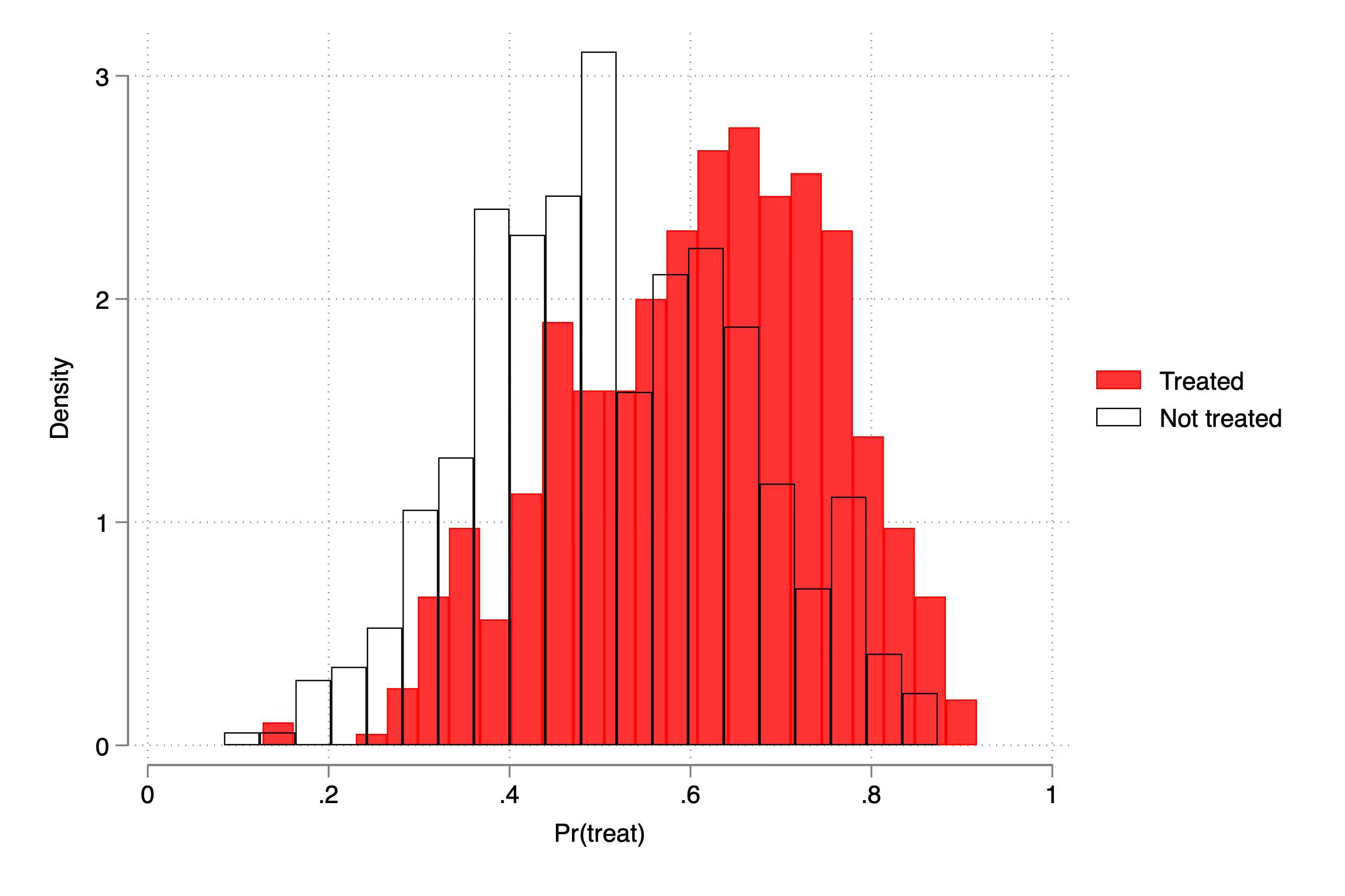
That’s good because for the double robust method I’m going to use below, I need there to be at least some units in the treatment and control across these covariates. And that is because conditional parallel trends is basically taking two groups that look different and more or less “fixing them” so that the parallel trends can operate through the covariates, even if parallel trends doesn’t hold for the two group comparisons on average. Here’s how we write down conditional parallel trends:
where b is the period just prior to treatment, or baseline, and t is post-treatment period, and the outcome terms are potential outcomes, specifically the untreated potential outcome. And we are saying that had the cities not built the football stadiums, their tax revenue would have evolved similar to the rural/suburban areas for those areas with comparable population sizes.
But then what does that mean in practice? It’s helpful to see code sometimes. Here’s what I did, with help from Kyle Butts when I couldn’t figure out why I was messing it up.
  * Generate fixed effect with control group making 10,000 more at baseline
  qui gen unit_fe = 40000 + 10000 * (treat == 0)

  * Generate Potential Outcomes with Baseline and Year Difference
  gen e = rnormal(0, 1500)
  qui gen     y0 = unit_fe        + 100 * age + 1000 * gpa + e if year == 1987
  qui replace y0 = unit_fe + 1000 + 150 * age + 1500 * gpa + e if year == 1988
  qui replace y0 = unit_fe + 2000 + 200 * age + 2000 * gpa + e if year == 1989
  qui replace y0 = unit_fe + 3000 + 250 * age + 2500 * gpa + e if year == 1990
  qui replace y0 = unit_fe + 4000 + 300 * age + 3000 * gpa + e if year == 1991
  qui replace y0 = unit_fe + 5000 + 350 * age + 3500 * gpa + e if year == 1992

  * Covariate-based treatment effect heterogeneity
  gen y1 = y0
  replace y1 = y0 + 1000 + 250 * age + 1000 * gpa if year >= 1991
I do two things in this. First, notice that Y(0) (the key potential outcome in difference-in-differences) grows by 1000 a year, but also grows by a different amount depending on a person’s baseline age and gpa. And then the second thing I did was introduce covariate-based heterogenous treatment effects. The interpretation is simpler than it looks: if a person never gets a college degree, then their earnings increase with age. But if they did get a college degree, then their earnings increases with age even more. It’s a statement that the impact of age on earnings differs depending on whether you’ve been treated or not. And in my case, it’s just a little modification so that we introduce that possibility.
Using this data generating process, the ATT in 1991 and 1992 are simply a summary of the individuals treated and their individual treatment effects. It depends on the draw because it varies with age and gpa which are somewhat random, but in the final calculation it’s going to be around $1620 in 1991 and $1620 in 1992 (i.e., no dynamic treatment effects).
Estimation with OLS
I will first present estimates from an OLS model in which I control for age, gpa, age squared, gpa squared and age-gpa interacted.
The code for this was this:
reg earnings treat##ib1990.year age gpa age_sq gpa_sq interaction, robust
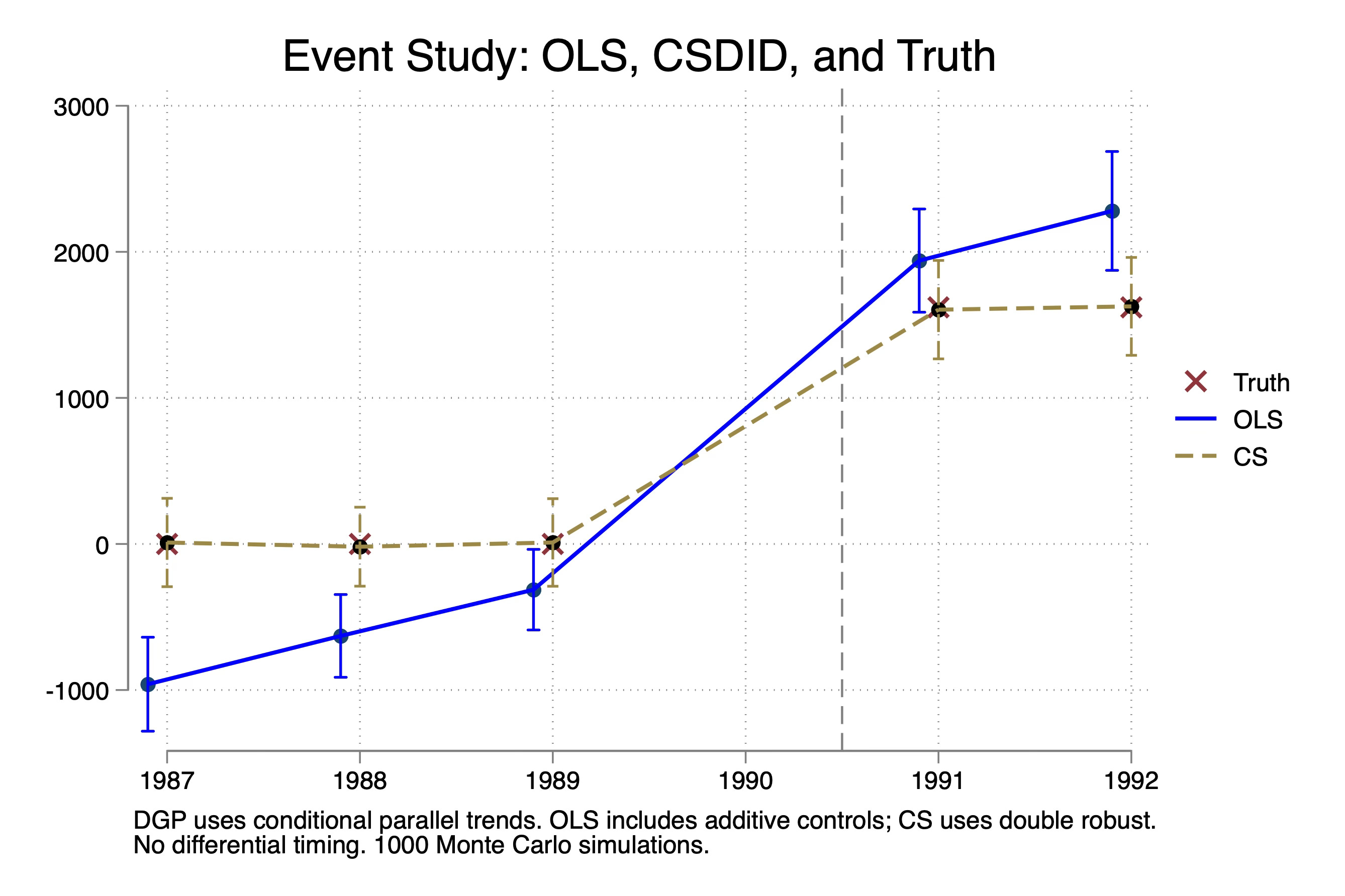
I ran this 1,000 times, each time estimating that equation and saving the coefficients on the treatment interaction indicators. I then plotted the mean and 95% upper and lower values from those 1,000 Monte Carlo trials. Here is what we find when we plot the event study plots overlaid with the “true effects”:
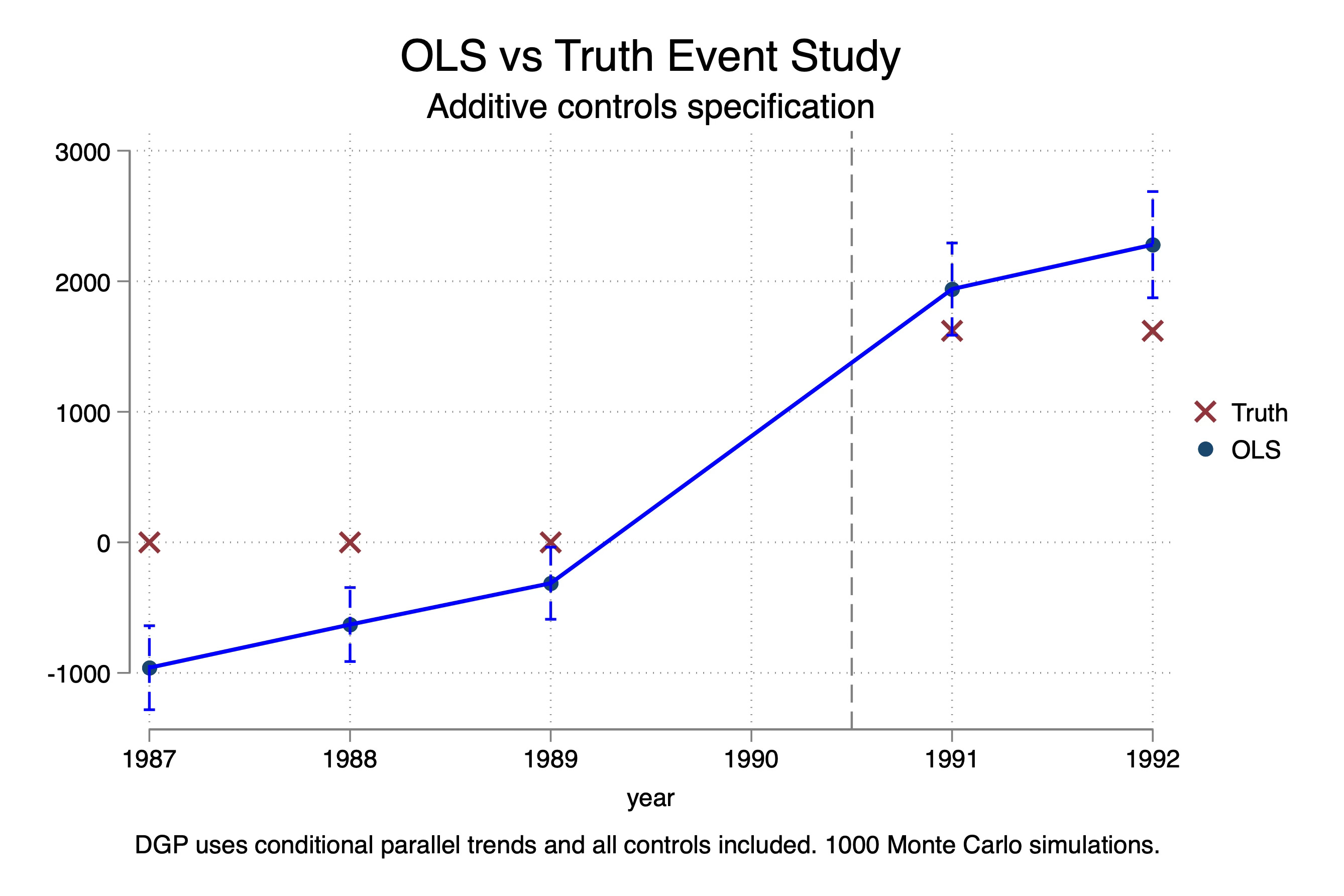
A few things stand out. First, there are no treatment effects until 1991. This is called “No Anticipation”, which is also required for difference-in-differences. Notice the X’s on 0 for 1987 to 1989. I should’ve put an X at 1990 but I forgot and I’m in too deep to turn around now, but there also wasn’t a treatment effect in 1990.
Second, notice there are no dynamic treatment effects. The effect pops up to around $1600 in 1991 and stays there.
Third, TWFE is biased. It’s biased on the pre-trends and it’s biased on the estimates of the treatment effects. Imagine now that you are running this regression and see pre-trends are not zero — you might despair. You don’t want to just see if your pre-trends are zero in principle; you want to know if your pre-trend estimates are unbiased, which is not the same thing. And here they are biased, not because you left out a covariate (in fact I included them), but because TWFE requires that the treatment effects be invariant to the covariates and it requires that Y(0) not grow covariates too. But in my case, that’s exactly what I did. The age-earnings profile when not treated was increasing each year, and the return to college varied with your age and high school GPA.
So this bias of TWFE is not coming from dynamics and it isn’t coming from differential timing. Rather, it’s coming from differential covariate trends and it’s coming from heterogenous treatment effects with respect to covariates.
Estimation with Double Robust (Callaway and Sant’Anna)
Next I look at the double robust method by Sant’Anna and Zhao. This is available in Stata and R as drdid but unfortunately you can’t use them to estimate event studies. To do that I use csdid (Callaway and Sant’Anna) which becomes Sant’Anna and Zhao when there isn’t differential. Speaking of Callaway and Sant’Anna (2021), as of today, they just passed 5,000 cites! Not bad for a paper published in 2021!
The double robust estimator has this expression:
As there is only one group, then just becomes the ATT for 1991 and 1992, as well as the three pre-treatment periods, 1987, 1988 and 1989. The interior terms are weights and the second outer term is the change in earnings from baseline to 1991 or 1992 (Delta Y) minus the predicted counterfactual for D=1 had they been treated. Double robust combined Abadie’s propensity score weighting method with Heckman, Ichimura and Todd’s earlier outcome regression method. You only need one of the models to be right in order for the method to be unbiased. And it is robust to treatment effect heterogeneity (which we have) and covariates that affect Y(0) (earnings without college) differently by year (which we also have). The command to estimate this uses -csdid-.
csdid earnings age gpa age_sq gpa_sq interaction, ivar(id) time(year) gvar(treat_date)
And I also ran this 1,000 times, saving the estimates on 1987, 1988, 1989, 1991 and 1992 and plotted them as an event study here:
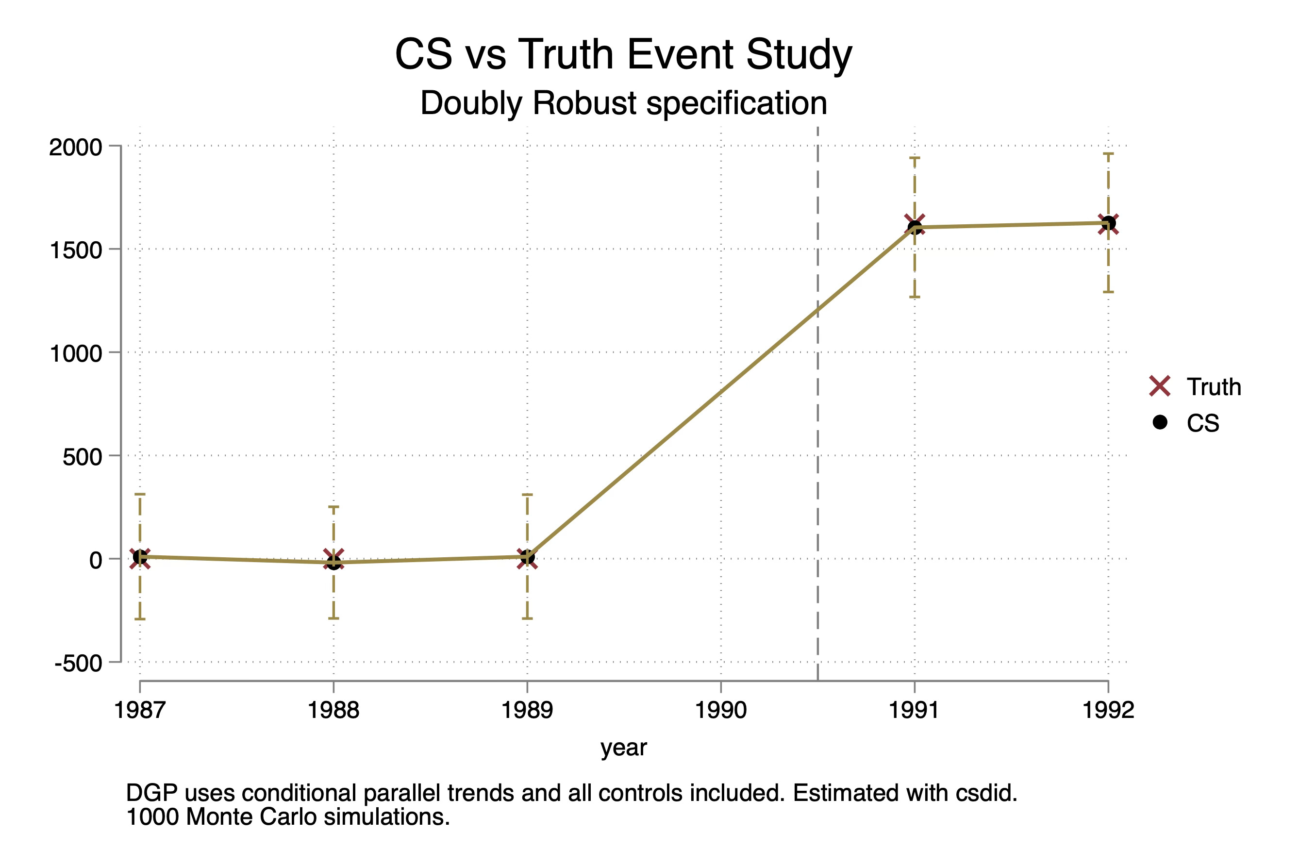
And as you can see, CS is unbiased estimating both pre-trend coefficients as well as the post-treatment ATT parameters for 1991 and 1992. Let’s now put them both on the same figure:
So why was OLS biased again?
This hopefully is a bit more helpful at illustrating the bias of OLS against a method that allows for heterogeneity with respect to covariates along two dimensions. First, there is treatment effect heterogeneity with respect to the covariates, as I said. This was captured here:
  * Covariate-based treatment effect heterogeneity
  gen y1 = y0
  replace y1 = y0 + 1000 + 250 * age + 1000 * gpa if year >= 1991
And then I allow for age and gpa to impact earnings in a world where you aren’t treated differently by which year it is. I did that here:
  * Generate fixed effect with control group making 10,000 more at baseline
  qui gen unit_fe = 40000 + 10000 * (treat == 0)

  * Generate Potential Outcomes with Baseline and Year Difference
  gen e = rnormal(0, 1500)
  qui gen     y0 = unit_fe        + 100 * age + 1000 * gpa + e if year == 1987
  qui replace y0 = unit_fe + 1000 + 150 * age + 1500 * gpa + e if year == 1988
  qui replace y0 = unit_fe + 2000 + 200 * age + 2000 * gpa + e if year == 1989
  qui replace y0 = unit_fe + 3000 + 250 * age + 2500 * gpa + e if year == 1990
  qui replace y0 = unit_fe + 4000 + 300 * age + 3000 * gpa + e if year == 1991
  qui replace y0 = unit_fe + 5000 + 350 * age + 3500 * gpa + e if year == 1992
And the way you should think about covariate-specific trends is really easy if you think about it as “age-earnings profile”, which was why I chose that example. Many economists will plot average earnings of workers across different ages. And all we mean here is that earnings can vary with age. And what I did was allow for age to have its own effect one earnings in a world where no one ever got a college degree. This is called “covariate-specific trends”, but it is important to note it is trends in Y(0), which if you recall, parallel trends is all about changes in Y(0) being the same for two groups. Here is a picture I made showing the average Y(0) across age.
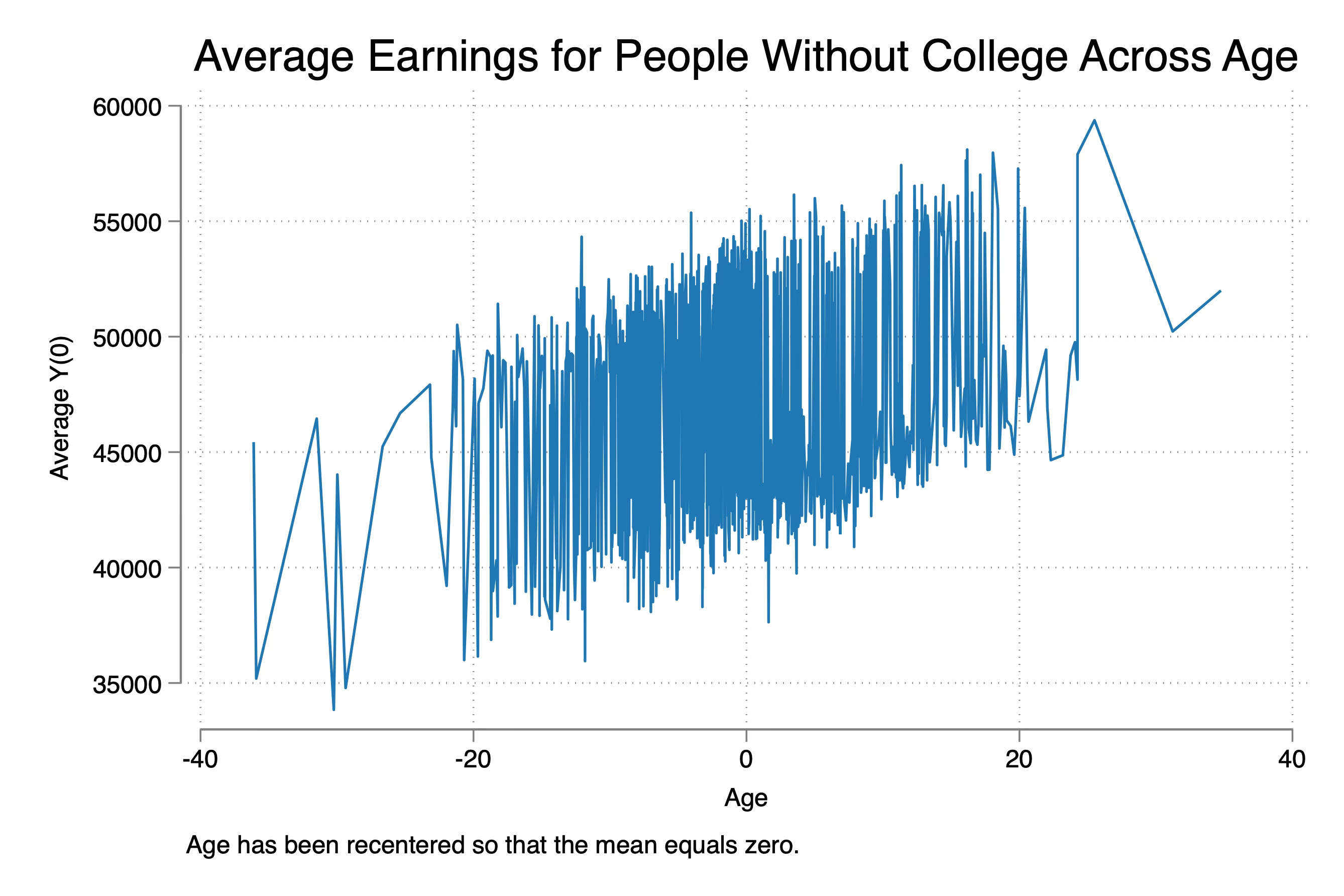
Well, as I said, the OLS model I ran required constant treatment effects and it required that age and earnings not have a trending effect on Y(0). Had neither been true in this data, then OLS would have been unbiased, but they weren’t true so it was.
Here we see once again that “exogeneity” imposes strong assumptions on the DGP. It imposes functional form assumptions on Y(0) and constant treatment effects. We could have used regression adjustment in a diff-in-diff to resolve this, but I just ran the simple OLS given that’s what 99.9999% of people do when they want to control for covariates. Here are the two event studies on top of each other.
Conclusion
So what did we learn? Well, one thing we learned is that selection on observables doesn’t break parallel trends, which was nice. That was this line of our code:
  * Treatment probability increases with age and decrease with gpa
  gen propensity = 0.3 + 0.3 * (age > 0) + 0.2 * (gpa > 0)
  gen treat = runiform() < propensity
So good news there. And then the second thing we learned is that you can get biased estimates on both pretrends and post-treatment ATT parameters using OLS even if you have all the correct controls. You would have to use regression adjustment, an Oaxaca-Blinder style version of difference-in-differences if you wanted to use OLS, which I think is what Jeff Wooldridge worked out for the differential timing case. But here I just used double robust transformations of simple difference-in-differences (differences in mean outcomes).
I hope this was helpful! So glad to finally have written this up. It’s burning a hole in my pocket for a long time. I was kind of trying to kill two birds with one stone, though, so I could cover both the selection and parallel trends material, but also introduce more information about biases of OLS with covariate-related heterogeneity in Y(0) and treatment effects. If you enjoyed this, check out the other entries I did on “Pedro’s Checklist” here, here, here, here, here, here.
See you around!
| * name: step4d.do | |
| * Selection on observables and conditional parallel trends | |
| clear all | |
| capture log close | |
| set seed 12345 | |
| ******************************************************************************** | |
| * Define dgp | |
| ******************************************************************************** | |
| cap program drop dgp | |
| program define dgp | |
| * 1,000 workers (25 per state), 40 states, 4 groups (250 per group), 6 years | |
| * First create the states | |
| quietly set obs 40 | |
| gen state = _n | |
| * Generate 1000 workers. These are in each state. So 25 per state. | |
| quietly expand 25 | |
| bysort state: gen worker=runiform(0,5) | |
| label variable worker "Unique worker fixed effect per state" | |
| quietly egen id = group(state worker) | |
| * Generate Covariates (Baseline values) | |
| gen age = rnormal(35, 10) | |
| gen gpa = rnormal(2.0, 0.5) | |
| * Center Covariates (Baseline) | |
| sum age, meanonly | |
| qui replace age = age - r(mean) | |
| sum gpa, meanonly | |
| qui replace gpa = gpa - r(mean) | |
| * Generate Polynomial and Interaction Terms (Baseline) | |
| gen age_sq = age^2 | |
| gen gpa_sq = gpa^2 | |
| gen interaction = age * gpa | |
| * Treatment probability increases with age and decrease with gpa | |
| gen propensity = 0.3 + 0.3 * (age > 0) + 0.2 * (gpa > 0) | |
| gen treat = runiform() < propensity | |
| * Generate the years | |
| quietly expand 6 | |
| sort state | |
| bysort state worker: gen year = _n | |
| * years 1987 -- 1992 | |
| replace year = 1986 + year | |
| * Post-treatment | |
| gen post = 0 | |
| qui replace post = 1 if year >= 1991 | |
| * Generate treatment dates | |
| gen treat_date = 0 | |
| replace treat_date = 1991 if treat==1 | |
| * Generate fixed effect with control group making 10,000 more at baseline | |
| qui gen unit_fe = 40000 + 10000 * (treat == 0) | |
| * Generate Potential Outcomes with Baseline and Year Difference | |
| gen e = rnormal(0, 1500) | |
| qui gen y0 = unit_fe + 100 * age + 1000 * gpa + e if year == 1987 | |
| qui replace y0 = unit_fe + 1000 + 150 * age + 1500 * gpa + e if year == 1988 | |
| qui replace y0 = unit_fe + 2000 + 200 * age + 2000 * gpa + e if year == 1989 | |
| qui replace y0 = unit_fe + 3000 + 250 * age + 2500 * gpa + e if year == 1990 | |
| qui replace y0 = unit_fe + 4000 + 300 * age + 3000 * gpa + e if year == 1991 | |
| qui replace y0 = unit_fe + 5000 + 350 * age + 3500 * gpa + e if year == 1992 | |
| * Covariate-based treatment effect heterogeneity | |
| gen y1 = y0 | |
| replace y1 = y0 + 1000 + 250 * age + 1000 * gpa if year >= 1991 | |
| * Treatment effect | |
| gen delta = y1 - y0 | |
| label var delta "Treatment effect for unit i (unobservable in the real world)" | |
| * Generate observed outcome based on treatment assignment | |
| gen earnings = y0 | |
| qui replace earnings = y1 if treat == 1 & year >= 1991 | |
| end | |
| ******************************************************************************** | |
| * Generate a sample | |
| ******************************************************************************** | |
| clear | |
| quietly dgp | |
| * Regression breaks | |
| reg earnings treat##ib1990.year age gpa age_sq gpa_sq interaction, robust | |
| * CSDID works | |
| csdid earnings age gpa age_sq gpa_sq interaction, ivar(id) time(year) gvar(treat_date) | |
| csdid_plot, group(1991) | |
| ******************************************************************************** | |
| * Monte-carlo simulation | |
| ******************************************************************************** | |
| cap program drop simulation | |
| program define simulation, rclass | |
| clear | |
| quietly dgp | |
| // True ATT | |
| gen true_att = y1 - y0 | |
| qui sum true_att if treat == 1 & year == 1991 | |
| return scalar att_1991 = r(mean) | |
| qui sum true_att if treat == 1 & year == 1992 | |
| return scalar att_1992 = r(mean) | |
| // CSDID | |
| qui csdid earnings age gpa age_sq gpa_sq interaction, ivar(id) time(year) gvar(treat_date) | |
| matrix b = e(b) | |
| return scalar cs_pre1987 = b[1,1] | |
| return scalar cs_pre1988 = b[1,2] | |
| return scalar cs_pre1989 = b[1,3] | |
| return scalar cs_post1991 = b[1,4] | |
| return scalar cs_post1992 = b[1,5] | |
| return scalar cs_att = (b[1,4] + b[1,5]) / 2 | |
| // OLS | |
| qui reg earnings treat##ib1990.year age gpa age_sq gpa_sq interaction, robust | |
| return scalar ols_pre1987 = _b[1.treat#1987.year] | |
| return scalar ols_pre1988 = _b[1.treat#1988.year] | |
| return scalar ols_pre1989 = _b[1.treat#1989.year] | |
| return scalar ols_post1991 = _b[1.treat#1991.year] | |
| return scalar ols_post1992 = _b[1.treat#1992.year] | |
| // OLS overall ATT | |
| qui reg earnings post##treat age gpa age_sq gpa_sq interaction, robust | |
| return scalar ols_att = _b[1.post#1.treat] | |
| end | |
| simulate att_1991 = r(att_1991) /// | |
| att_1992 = r(att_1992) /// | |
| cs_pre1987 = r(cs_pre1987) /// | |
| cs_pre1988 = r(cs_pre1988) /// | |
| cs_pre1989 = r(cs_pre1989) /// | |
| cs_post1991 = r(cs_post1991) /// | |
| cs_post1992 = r(cs_post1992) /// | |
| cs_att = r(cs_att) /// | |
| ols_pre1987 = r(ols_pre1987) /// | |
| ols_pre1988 = r(ols_pre1988) /// | |
| ols_pre1989 = r(ols_pre1989) /// | |
| ols_post1991 = r(ols_post1991) /// | |
| ols_post1992 = r(ols_post1992) /// | |
| ols_att = r(ols_att), /// | |
| reps(100) seed(12345): simulation | |
| // Summarize results | |
| sum | |
| // Store results | |
| save ./step4d.dta, replace | |
| ******************************************************************************** | |
| * Plot results | |
| ******************************************************************************** | |
| use ./step4d.dta, clear | |
| * Calculate means and standard deviations for OLS variables | |
| summarize ols_pre1987 | |
| local ols_pre1987_mean = r(mean) | |
| local ols_pre1987_sd = r(sd) | |
| summarize ols_pre1988 | |
| local ols_pre1988_mean = r(mean) | |
| local ols_pre1988_sd = r(sd) | |
| summarize ols_pre1989 | |
| local ols_pre1989_mean = r(mean) | |
| local ols_pre1989_sd = r(sd) | |
| summarize ols_post1991 | |
| local ols_post1991_mean = r(mean) | |
| local ols_post1991_sd = r(sd) | |
| summarize ols_post1992 | |
| local ols_post1992_mean = r(mean) | |
| local ols_post1992_sd = r(sd) | |
| * Calculate means and standard deviations for CSDID variables | |
| summarize cs_pre1987 | |
| local cs_pre1987_mean = r(mean) | |
| local cs_pre1987_sd = r(sd) | |
| summarize cs_pre1988 | |
| local cs_pre1988_mean = r(mean) | |
| local cs_pre1988_sd = r(sd) | |
| summarize cs_pre1989 | |
| local cs_pre1989_mean = r(mean) | |
| local cs_pre1989_sd = r(sd) | |
| summarize cs_post1991 | |
| local cs_post1991_mean = r(mean) | |
| local cs_post1991_sd = r(sd) | |
| summarize cs_post1992 | |
| local cs_post1992_mean = r(mean) | |
| local cs_post1992_sd = r(sd) | |
| summarize att_1992 | |
| local true_att_1991 = r(mean) | |
| summarize att_1991 | |
| local true_att_1992 = r(mean) | |
| * Create a new dataset for plotting | |
| clear | |
| set obs 5 | |
| * Define the years | |
| gen year = 1987 + _n - 1 | |
| replace year = 1991 if _n == 4 | |
| replace year = 1992 if _n == 5 | |
| * True ATT values | |
| gen truth = 0 | |
| replace truth = `true_att_1991' if year == 1991 | |
| replace truth = `true_att_1992' if year == 1992 | |
| * OLS means and confidence intervals | |
| gen ols_mean = . | |
| gen ols_ci_lower = . | |
| gen ols_ci_upper = . | |
| replace ols_mean = `ols_pre1987_mean' in 1 | |
| replace ols_mean = `ols_pre1988_mean' in 2 | |
| replace ols_mean = `ols_pre1989_mean' in 3 | |
| replace ols_mean = `ols_post1991_mean' in 4 | |
| replace ols_mean = `ols_post1992_mean' in 5 | |
| replace ols_ci_lower = ols_mean - 1.96 * `ols_pre1987_sd' in 1 | |
| replace ols_ci_lower = ols_mean - 1.96 * `ols_pre1988_sd' in 2 | |
| replace ols_ci_lower = ols_mean - 1.96 * `ols_pre1989_sd' in 3 | |
| replace ols_ci_lower = ols_mean - 1.96 * `ols_post1991_sd' in 4 | |
| replace ols_ci_lower = ols_mean - 1.96 * `ols_post1992_sd' in 5 | |
| replace ols_ci_upper = ols_mean + 1.96 * `ols_pre1987_sd' in 1 | |
| replace ols_ci_upper = ols_mean + 1.96 * `ols_pre1988_sd' in 2 | |
| replace ols_ci_upper = ols_mean + 1.96 * `ols_pre1989_sd' in 3 | |
| replace ols_ci_upper = ols_mean + 1.96 * `ols_post1991_sd' in 4 | |
| replace ols_ci_upper = ols_mean + 1.96 * `ols_post1992_sd' in 5 | |
| * CSDID means and confidence intervals | |
| gen csdid_mean = . | |
| gen csdid_ci_lower = . | |
| gen csdid_ci_upper = . | |
| replace csdid_mean = `cs_pre1987_mean' in 1 | |
| replace csdid_mean = `cs_pre1988_mean' in 2 | |
| replace csdid_mean = `cs_pre1989_mean' in 3 | |
| replace csdid_mean = `cs_post1991_mean' in 4 | |
| replace csdid_mean = `cs_post1992_mean' in 5 | |
| replace csdid_ci_lower = csdid_mean - 1.96 * `cs_pre1987_sd' in 1 | |
| replace csdid_ci_lower = csdid_mean - 1.96 * `cs_pre1988_sd' in 2 | |
| replace csdid_ci_lower = csdid_mean - 1.96 * `cs_pre1989_sd' in 3 | |
| replace csdid_ci_lower = csdid_mean - 1.96 * `cs_post1991_sd' in 4 | |
| replace csdid_ci_lower = csdid_mean - 1.96 * `cs_post1992_sd' in 5 | |
| replace csdid_ci_upper = csdid_mean + 1.96 * `cs_pre1987_sd' in 1 | |
| replace csdid_ci_upper = csdid_mean + 1.96 * `cs_pre1988_sd' in 2 | |
| replace csdid_ci_upper = csdid_mean + 1.96 * `cs_pre1989_sd' in 3 | |
| replace csdid_ci_upper = csdid_mean + 1.96 * `cs_post1991_sd' in 4 | |
| replace csdid_ci_upper = csdid_mean + 1.96 * `cs_post1992_sd' in 5 | |
| twoway (scatter truth year, mcolor(maroon) msize(6-pt) msymbol(lgx) mlabcolor() mfcolor(cranberry) mlwidth(medthick)) /// | |
| (scatter ols_mean year, mcolor(navy) msize(6-pt)) /// | |
| (line ols_mean year, lcolor(blue) lwidth(medthick)) /// | |
| (rcap ols_ci_lower ols_ci_upper year, lcolor(blue) lpattern(dash)), /// | |
| title("OLS vs Truth Event Study") /// | |
| subtitle("Additive controls specification") /// | |
| note("DGP uses conditional parallel trends and all controls included. 1000 Monte Carlo simulations.") /// | |
| legend(order(1 "Truth" 2 "OLS")) /// | |
| xline(1990.5, lpattern(dash) lcolor(gray)) | |
| graph export "/Users/scunning/Library/CloudStorage/Dropbox-MixtapeConsulting/scott cunningham/0.1 Mixtape Consulting/Substack/Code/step4d_ols.png", as(png) name("Graph") replace | |
| twoway (scatter truth year, mcolor(maroon) msize(6-pt) msymbol(lgx) mlabcolor() mfcolor(cranberry) mlwidth(medthick)) /// | |
| (scatter csdid_mean year, mcolor(saddle) msize(6-pt)) /// | |
| (line csdid_mean year, lcolor(brown) lwidth(medthick)) /// | |
| (rcap csdid_ci_lower csdid_ci_upper year, lcolor(brown) lpattern(dash)), /// | |
| title("CS vs Truth Event Study") /// | |
| subtitle("Doubly Robust specification") /// | |
| note("DGP uses conditional parallel trends and all controls included. Estimated with csdid." "1000 Monte Carlo simulations.") /// | |
| legend(order(1 "Truth" 2 "CS")) /// | |
| xline(1990.5, lpattern(dash) lcolor(gray)) | |
| graph export "/Users/scunning/Library/CloudStorage/Dropbox-MixtapeConsulting/scott cunningham/0.1 Mixtape Consulting/Substack/Code/step4d_cs.png", as(png) name("Graph") replace | |
| * Shift years slightly to avoid overlap | |
| gen year_ols = year - 0.1 | |
| gen year_csdid = year | |
| * Plotting | |
| twoway (scatter truth year, mcolor(maroon) msize(6-pt) msymbol(lgx) mlabcolor() mfcolor(cranberry) mlwidth(medthick)) /// | |
| (scatter ols_mean year_ols, mcolor(navy) msize(6-pt)) /// | |
| (line ols_mean year_ols, lcolor(blue) lwidth(medthick)) /// | |
| (rcap ols_ci_lower ols_ci_upper year_ols, lcolor(blue)) /// | |
| (scatter csdid_mean year_csdid, mcolor(saddle) msize(6-pt)) /// | |
| (line csdid_mean year_csdid, lcolor(brown) lwidth(medthick) lpattern(dash)) /// | |
| (rcap csdid_ci_lower csdid_ci_upper year_csdid, lcolor(brown) lpattern(dash)), /// | |
| title("Event Study: OLS, CSDID, and Truth") /// | |
| note("DGP uses conditional parallel trends. OLS includes additive controls; CS uses double robust." "No differential timing. 1000 Monte Carlo simulations.") /// | |
| legend(order(1 "Truth" 3 "OLS" 6 "CS") /// | |
| label(1 "Truth" ) /// | |
| label(2 "OLS" ) /// | |
| label(3 "CS" )) /// | |
| xline(1990.5, lpattern(dash) lcolor(gray)) | |
| * Export the graph | |
| graph export "/Users/scunning/Library/CloudStorage/Dropbox-MixtapeConsulting/scott cunningham/0.1 Mixtape Consulting/Substack/Code/step4d_combined.png", as(png) name("Graph") replace | |