


Selection on Y(0) and Parallel Trends: Anticipating Step (4) in Pedro's Diff-in-Diff Checklist
Selection on Y(0) and Parallel Trends: Anticipating Step (4) in Pedro's Diff-in-Diff Checklist

People select into a treatment based on any number of reasons. For instance, they could end up taking a polio vaccine because they were in a study where the polio vaccine was randomized, which is similar to saying they were assigned to the treatment because of an instrument. But sometimes it could be because of observable covariates, like their age, that we collapse into a propensity score. Or maybe they took the polio vaccine because the government had a contest, and if you were born after April 18th, you got it, and you were born on April 18th or sooner, you didn’t — what we call a running variable.
Each treatment assignment mechanism implies a particular set of assumptions that can be operationalized into an estimator. If you were randomized, then you do simple comparison in mean outcomes between the vaccinated group and the non-vaccinated group. And if there was non-compliance, you use instrumental variables based on that lottery. If it’s based on observables, you might use propensity scores, and if it was based on a running variable, you might use local polynomial regressions. Point is, the treatment assignment mechanism drives your choices, and cannot be skipped.
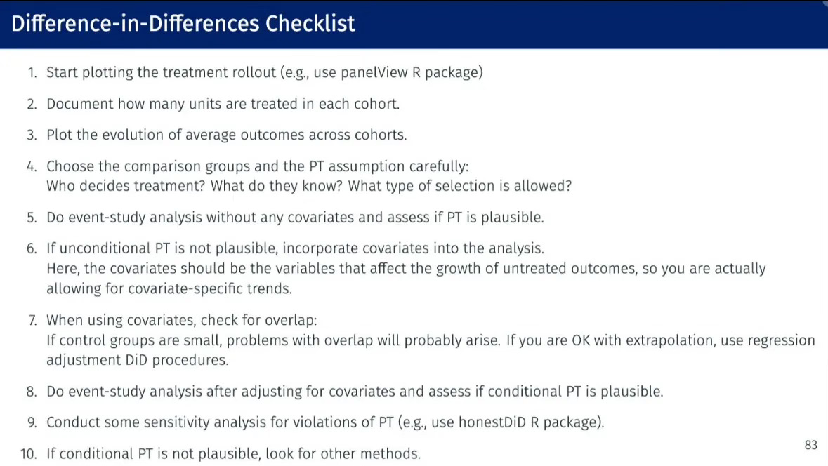
But then what is the treatment assignment mechanism that justifies our belief in parallel trends such that were are then in the clear to use difference-in-differences? If we are following Pedro’s diff-in-diff checklist (here are the previous step 1, step 2, and step 3 substack posts), then we get to step 4 which is entirely about this question of the treatment assignment mechanism. Look closely:
"Choose the comparison group and the parallel trends assumption carefully: who decides treatment? What do they know? What type of selection is allowed?"
I don’t think we can really dive into step 4 without trying to understand a little about treatment assignment mechanisms that do and do not justify parallel trends. So to do that, I am going to just cover a little bit of a 2023 working paper by Pedro Sant'Anna, Dalia Ghanem and Kaspar Wüthrich, in which they examine the various types of selection processes that justify our parallel counterfactual trends hypothesis. There are several selection mechanisms they consider, so I’m only going to focus on the first one which is selection based on untreated potential outcomes, or Y(0). And I’ll do it using a simulation again.
Selection on untreated potential outcomes in a cross-section
What do I mean when I say “selection on untreated potential outcomes”? Selection on untreated potential outcomes is when units decide to participate based on expected untreated potential outcomes relative to some threshold. And to illustrate we will first just show this in a simulation using a simple cross-section.
To be concrete, let’s assume that the treatment is a food stamps program (i.e., SNAP) and our potential outcomes will measure earnings. For the sake of simplicity, we want to know the causal effect of being enrolled on SNAP on earnings. And we will assume that a person enrolls if their untreated potential outcome falls below some earnings’ threshold of $100. Let me give an abstract example in Stata code. We will generate a dataset with 1 million people in it.
clear all
set seed 1
set obs 1000000

gen id = _n
gen y0 = 100 + rnormal(0,20)
gen y1 = 150 + rnormal(0,15)
gen delta = y1-y0
su delta // ATE is 49.97953
Now these few lines simply generated potential outcomes, Y(1) and Y(0), for each of our million people. The mean of Y(1) is 150, the mean of Y(0) is 100, so the ATE is 50 with individual treatment effects ranging from -68 to 177. But notice, no treatment yet.
Selection into treatment based on Y(0) would mean something as simple as this:
* selection based on y0: y1 _||_ D

gen 	d=0
replace d=1 if y0<=100

* Create the aggregate conditional causal effects
egen ate = mean(delta)
egen att = mean(delta) if d==1
egen atu = mean(delta) if d==0
su ate // ATE is 49.97953
su atu // ATI is 33.97148
su att // ATT is 65.94704
Interestingly, when selection into the treatment is based on Y(0), but not Y(1), then the mean of Y(0) will differ by the treatment group, but not Y(1). And you can see that here:
* Check for independence with respect to y0
summarize y0 if d==0 // 115.9762
summarize y0 if d==1 // 84.05979

* check for independence with respect to y1

summarize y1 if d==0 // 149.9476
summarize y1 if d==1 // 150.0068
Selection on untreated potential outcomes in two periods
But that was for independence. What we want to know is how this selection mechanism affects the change in Y(0) for the treatment and control group, and to generate that, we need to generate a simple two period dataset in which selection into the sample happens when Y(0) falls below some threshold.
* selection_outcomes.do: selection into treatment based on Y(0)

  * Set up
  clear all
  set seed 2

  * First create the states
  quietly set obs 40
  gen state = _n

  * Generate 1000 workers. These are in each state. So 25 per state.
  expand 25
  bysort state: gen unit_fe=runiform(1,1000)
  label variable unit_fe "Unique worker fixed effect per state"
  egen id = group(state unit_fe)

  * Generate pontential outcomes
  gen y0 = unit_fe + rnormal(0,10)
First, we generated 40 states, 1,000 workers with 25 per state, and 2 years of data with worker fixed effects drawn from a uniform distribution. The baseline year is 1990; the post-treatment year is 1991. And notice that our untreated potential outcome is simply an individual worker’s fixed effect plus some random noise.
Next we want to show the selection into the treatment. Recall that a person selects into the treatment when their untreated potential outcome (i.e., earnings at baseline) falls “too low”. For this, I’ll say that if your baseline earnings is at the 25th percentile or lower, you qualify for SNAP.
* Determine treatment status in 1990
  su y0, detail
  gen treat = 0
  replace treat = 1 if y0 < `r(p25)'

  * Generate the years
  expand 2
  sort state
  bysort state unit_fe: gen year = _n
  gen n = year
  replace year = 1990 if year == 1
  replace year = 1991 if year == 2

  * Post-treatment
  gen post = 0
  replace post = 1 if year == 1991

  replace y0 = y0 + 1000 if year == 1991
Once I generated the treatment, I just added a second year and then created dummies for the post period, as well as created a trend in the potential outcome equal to +$1,000 from 1990 to 1991.
Next we need to generate the treated potential outcome, Y(1), which we will use both to figure out the average treatment effects, but also to ultimately assign treated units to Y(1) if treated in a given year and Y(0) otherwise. Let’s do that now.
  gen y1 = y0
  replace y1 = y0 + 7500 if year==1991

  * Treatment effect
  gen delta = y1 - y0
  label var delta "Treatment effect for unit i (unobservable in the real world)"

  sum delta if post == 1, meanonly
  gen ate = `r(mean)' // $7,500
  sum delta if treat==1 & post==1, meanonly
  gen att = `r(mean)' // $7,500

  * Generate observed outcome based on treatment assignment
  gen         earnings = y0
  qui replace earnings = y1 if post == 1 & treat == 1
The ATE and the ATT are both in this case $7,500 and that’s because y1 is equal to y0 + 7500, which is $7,500. There are no covariates in this example, and as such, the average treatment effects are the same for the treated, the untreated and the whole sample. Then we used the switching equation and assigned a unit to have their earnings equal Y(0) if they were either in the control group or it was the baseline. Otherwise they were assigned to Y(1) which was the treatment group in the post treatment period.
Selection on Y(0) and Parallel Trends
Now we want to just see how our treatment assignment mechanism — i.e., when a person’s baseline earnings was below the 25th percentile — created parallel trends. To illustrate this, I’ll run this code then show the output.
  * Illustrate parallel trends assumption
  su y0 if treat==1 & post==0
  gen ey0_10 = `r(mean)'
  su y0 if treat==1 & post==1
  gen ey0_11 = `r(mean)'
  su y0 if treat==0 & post==0
  gen ey0_00 = `r(mean)'
  su y0 if treat==0 & post==1
  gen ey0_01 = `r(mean)'

  gen parallel_trends = (ey0_11 - ey0_10) - (ey0_01 - ey0_00)

  reg y0 post##treat, robust

  su parallel_trends
Notice that I can calculate the parallel trends as either four averages and three subtractions on y0, or I could just run a regression of y0 onto a treatment dummy, a post dummy and an interaction. When I do I get this output.
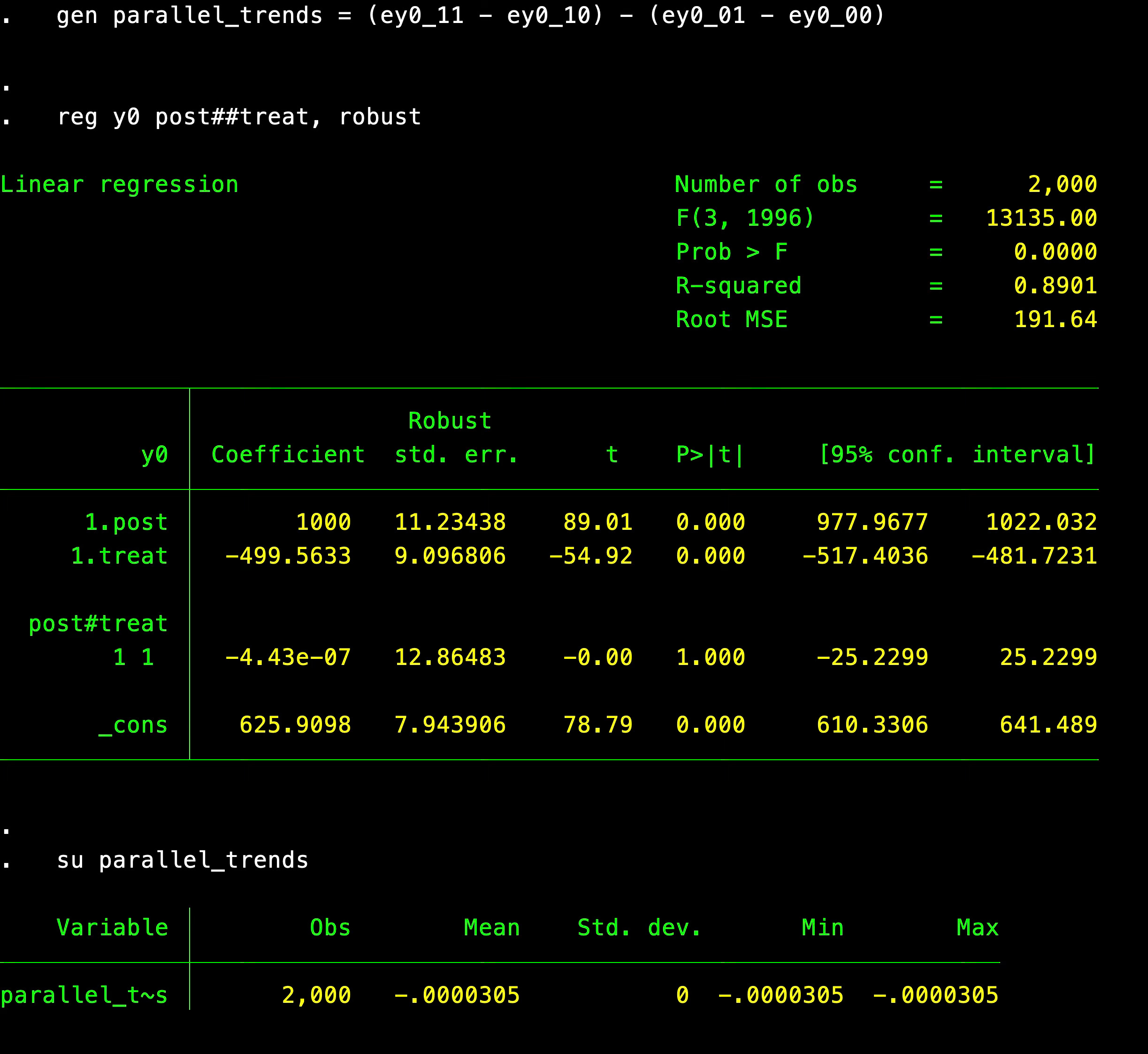
You can see here that when selection into the treatment was based on Y(0), i.e., the baseline untreated outcome, then it generated parallel trends. This happened because the potential outcome Y(0) was not based on treatment status; treatment status was based on it.
I encourage you to try to play around with this yourself too, but for now, let’s look at the difference-in-differences result. Recall what DiD identifies:
And since the ATT is $7,500 and we just showed that the parallel trends bias is zero, then our diff-in-diff estimate will be around $7,500. The code for that is here:
  * Diff-in-diff
  su earnings if treat==1 & post==0
  gen ey_10 = `r(mean)'
  su earnings if treat==1 & post==1
  gen ey_11 = `r(mean)'
  su earnings if treat==0 & post==0
  gen ey_00 = `r(mean)'
  su earnings if treat==0 & post==1
  gen ey_01 = `r(mean)'

  gen did = (ey_11 - ey_10) - (ey_01 - ey_00)

  reg earnings post##treat, robust

  su did att
And the output for it is here:
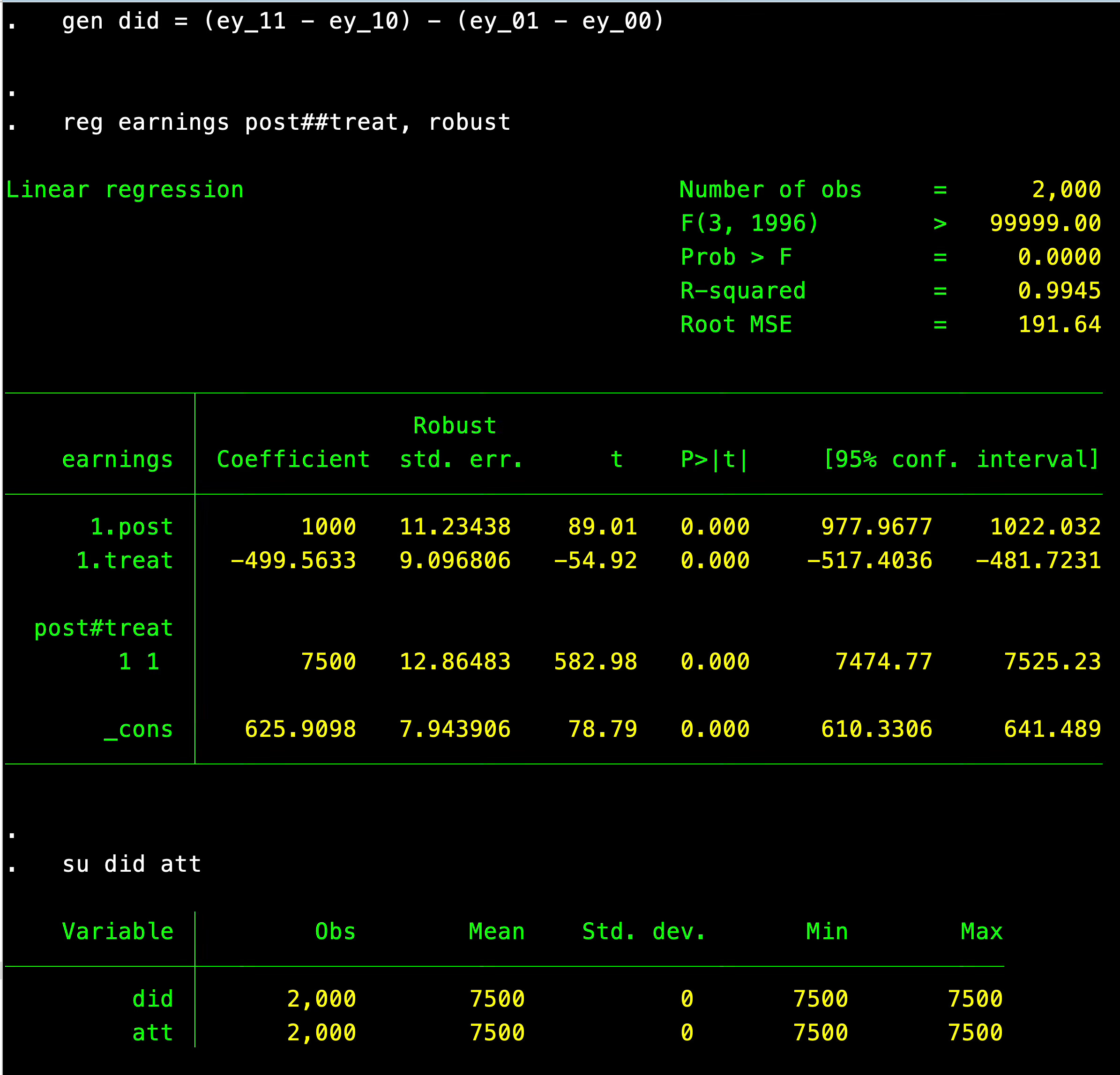
And sure enough, the diff-in-diff estimate of the average effect of SNAP on SNAP participants’ earnings was $7,500, which we knew was the ATT since we generated the data.
Conclusion
Before we dive into step 4 and figure out what that entails, I am just going to go through this “Selection and Parallel Trends” paper a little at a time until we feel like we know the types of treatment assignment mechanisms that are consistent with parallel trends and those that are not. And the one that is is when selection is based on Y(0). As we saw with our simple numerical example, parallel trends held, despite selection based on the baseline potential outcome. But what does it mean?
It means that if you think people are looking at their earnings in the baseline and thinking to themselves “my earnings are too low; I will choose the treatment”, but they are not thinking about the causal effect of the treatment (just Y(0), not Y(1)-Y(0) in other words), then this is consistent with parallel trends, which is consistent with using difference-in-differences. Now this doesn’t give us an answer yet to step 4, but hopefully it will soon!