

Claude Code 26: Multiple Agents Auditing Your Callaway and Sant'Anna Diff-in-Diff (Part 2)
Exploring Researcher Degrees of Freedom ("Non-Standard Errors") with 15 Agents

This is part of my ongoing series on using Claude Code for practical applied empirical work valued by the quantitative social sciences. And this is specifically going with a difference-in-differences (DiD) idea that I started the other day which you can find here:

In part 1, the DiD thread started with a slightly different experiment of illustrating pure “hostile critic audits of your code”, but when I looked at the data this week, I decided to change it as I became less interested in illustrating the “referee2” auditor when I saw certain things — at least not yet. So I have decided to pivot this DiD series into a slightly different direction — a systematic investigation of what AI agents actually do when you hand them a real empirical problem and walk away, which is a variation on the “multi-analyst design” that Nick Huntington-Klein and others have been working on these last few years. If you're just joining, you can learn a little by reviewing the last post and video, but you also might be able to just start here as in this video, I go over the experiment that I did before the video started (running 15 sub agents to do the replication). But the first video gives you the intuition for why I started running multiple agents in the first place.
Finally, the paper being replicated is this AEJ: Policy by Dias and Fontes in which a Brazilian mental health reform’s effect on municipality-level homicide rates was studied using difference-in-differences, specifically the de Chaisemartin and D’Haultfoueille (2020, AER). But in this, I use the Callaway and Sant’Anna method, both of which are often used with staggered treatment adoption.
Thank you again everyone for your support of the substack. If you are a paying subscriber, thank you! If you are not, enjoy! The Claude Code series remains free but after a few days, it will go behind a paywall. So if you are just joining, consider becoming a paying subscriber so that you can read the other 25 posts I’ve done on Claude Code since early to mid December of 2025. The prices is $5/month!
The previous Claude Code video walkthroughs have been pretty long — often 60 to 90 minutes. And in this one, I tried to rein it in so that it’s at least somewhat watchable. But it still came in at 38 minutes. And that required pausing it, too, leaving us with a bit of a cliffhanger. Still, I will post the third part of the series next week, so let me for now just walk you through this one.
As I said above, if you watched the first video in this sequence, you saw me run a version of today’s experiment. But leading into today’s video, I peaked at the results, and I just decided I was more interested in a different thing than I originally did so last night I redid the whole thing (with Claude Code’s help). The bones are somewhat the same in that I am evaluating sub-agent driven coding up in three languages (python, R and Stata) of five packages (csdid, csdid2, did, differences, diff-diff). So those parts are the same. And as I said, they all run Callaway and Sant’Anna on the Brazilian municipality data.
But I decided to tighten the isolation protocol (I’ll explain that) after reviewing the output from the part 1 experiment. I also adjusted the instructions, and expanded the forensic analysis I do afterward. This led to a 52 page “beautiful deck” (build using the /compiledeck skill I use constantly which is based on my “rhetoric of decks” essay I feed to Claude Code also when creating decks). So think of everything now going forward as a revision and an extension of the original version.
Discretion and Non-Standard Errors in Difference-in-Differences Estimation
As I mentioned, there is a literature I have been super interested in for several years now which is often called the “multi-analyst design”. As I understand it, this literature began with Silberzahn et al. in 2018, who gave 29 research teams the same dataset and the same question — whether dark-skinned soccer players receive more red cards. The estimates ranged from strongly negative to strongly positive. Same data, same question, wildly different answers.
Nick Huntington-Klein and coauthors did something similar in 2021. They recruited seven economists to independently replicate two published causal results. Each got the same data and the same research question. No two replicators reported the same sample size. The standard deviation across their estimates was three to four times the typical reported standard error. And I found that super interesting for a few reasons. One, the standard errors we report are meant to approximate the standard deviation in the sampling distribution of estimator. And yet Nick’s team was reporting a standard deviation that was four times larger than the mean standard error, which means they were quantifying a source of uncertainty that is not remotely what standard errors are measuring. And the other thing I was fascinated by was the idea that the confidence interval from any individual analysis dramatically understates the true uncertainty about the result as what if we had given this same project to someone else? Would they have made the same decisions? It depended on the number of researcher degrees of freedom and their relevance, as inputs, in the final estimates.
Then there’s the Journal of Finance paper from Menkveld and coauthors in 2024, which coined the term “non-standard errors” — the variation they document definitely does not and cannot from sampling (not even bootstrapping) but from an accumulation of small analytical choices. And Borjas and Breznau in 2025, who found that with an immigration question, researcher ideology predicted the sign of the effect.
The common thread is that when researchers have discretion, then you can get spreading out of estimates even with the same raw dataset, the same goal, the same research question, the same groups of people doing the estimation. Give smart, well-trained people the same data and the same question, and the spread of answers is large — often larger than any individual analyst’s reported uncertainty. The variation isn’t errors, or p-hacking, too — it’s coming from researcher discretion, and biases.
Three things I wanted to learn
So, now this project is trying to do three things at once, and I want to explain what that is now.
First, I want to know whether running the same analysis with multiple independent AI agents could serve as a robustness audit. That’s my referee2 code audit. But I’ve extended and integrated that into both DiD analysis to check for the spread of estimates across independent runs to see if it tells you something useful about how sensitive your conclusions are to the choices being made under the hood. I think that’s in and of itself interesting, and it’s not really the same thing as what my referee2 code auditor is doing.
Second, I wanted to test whether AI agents could approximate a many-analysts design like Nick’s and others. This is sort of connected to a different series I’ve been doing where I have been replicating studies using Claude Code and OpenAI gpt-4o-mini to see if you can use one-shot classification with consumer LLMs. You can see the fifth of that five-part series here (and if you click through you’ll find the other four):
I thought these were interesting illustrations of what you can do with Claude Code, but they also were interesting applications of LLMs for classification too. The comparison was to a trained RoBERTa model based on hiring ~7 student workers to read and classify ~7500 speeches and then train another 200,000 using RoBERTa. I wanted to see if you could do it much less expensively using gpt-4o-mini at OpenAI with batch requests in one-shots. And I did that because the human version is powerful but expensive — you have to recruit analysts, coordinate them, wait for results. And the frontier models continue to get cheaper and better, so if you can do them, you can do things really inexpensively without lost gains. Well it’s the same here. If AI agents produce qualitatively similar patterns of variation, that’s a cheap diagnostic tool. Maybe we could do them, report forest plots, in addition to auditing our code and non-standard errors could become something we report. So that is the other part of this exercise
Third, I wanted to map the specific points where discretion enters a staggered DiD project. Not discretion in general — I wanted a concrete inventory. Which decisions do analysts agree on? Which ones generate all the variation? Where exactly does the uncertainty live? So that’s what this is about.
What the agents actually saw
So, consistent with the many-analyst design, all of the AI agents that Claude Code made were given the same dataset, the same question, the same estimator, and many other discretionary decisions completely made for them. So let me review that now.
The dataset covers 5,476 Brazilian municipalities. The treatment is the rollout of CAPS mental health centers — Centros de Atenção Psicossocial — which were adopted by different municipalities at different times between 2002 and 2016. The outcome is homicide rates. And there are roughly twenty potential covariates: economic variables like GDP, poverty, and inequality; demographic variables like population, age structure, and literacy; health variables like spending and professional counts; and geographic variables like temperature, altitude, and distance to the state capital.
The staggered adoption makes this a natural setting for the Callaway and Sant’Anna estimator. And the covariate set is genuinely ambiguous — reasonable analysts could disagree about which variables satisfy the conditional parallel trends assumption and which ones are mediators that should be excluded. See section 4.2 of our JEL to learn more about conditional parallel trends.
So with Claude Code, we wrote a single instructions file — a short markdown document — and gave each agent nothing else. The instructions specified: use the Callaway and Sant’Anna estimator, use a universal base period (Roth 2026) with not-yet-treated control group, and — and this is the primary discretionary point [I tried to make it the only one too, but I’m still wondering if I missed something] — then to select covariates which would satisfy conditional parallel trends and common support. This is a major thing because pretty much every DiD uses covariates, and the purpose of that in DiD is, as I said earlier, to satisfy an untestable assumption called “conditional parallel trends”. So, even though conditional parallel trends can be written down as a coherent mathematical object, in practice no one knows what it is. And so this is a discretionary node in the chain of decision points that take you from the raw data to the estimates, and in my own analysis, the inclusion of covariates can play massive roles in estimation, sometimes even flipping signs!
Then the agents had to produce a balanced event study from four periods before treatment to four periods after, report a simple ATT averaged over the post-treatment periods, and document every decision in structured checkpoint files.
But as I said, the instructions did not say which covariates to use, which doubly robust variant to choose, or how to handle any data issues. Those were left to each agent’s judgment.
Fifteen agents, five packages, three languages
I ran three independent agents on each of five packages: differences and diff-diff in Python, did in R, and csdid and csdid2 in Stata. Fifteen total runs over 3 language-specific packages.
Each agent was a fresh Claude session launched via claude -p with no shared memory, no conversation history, and no access to any other agent’s work. Each saw exactly two files: the shared instructions and a one-page appendix naming its assigned package.
The isolation protocol was strict. My own reference code was moved to a hidden directory. Each agent worked in an isolated temp directory. All prior output was archived outside the project before each new run. Output was moved to its final location only after the agent exited. There was no way for one agent to see what another had done.
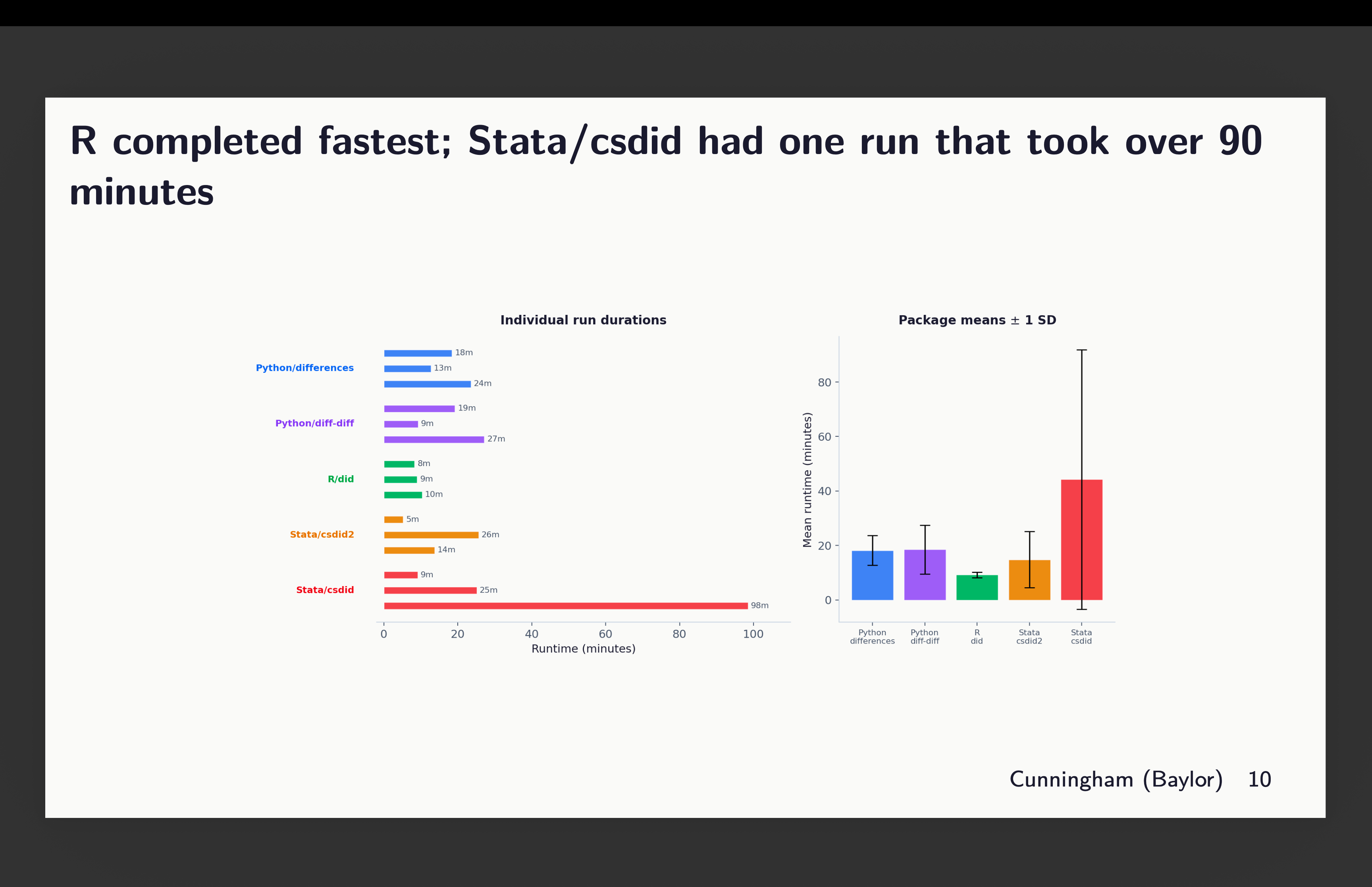
Here was the runtime. Pedro and Brant will be happy to learn that their R package was the fastest. And csdid in Stata had a huge outlier (100 minutes) which caused its mean to get larger than the rest, with a larger standard deviation.
What they agreed on was unanimous
This is the first result that surprised me, and it comes before any event study or ATT estimate.
All fifteen agents agreed on every structural decision. Control group: not-yet-treated, 15 out of 15. Base period: universal, 15 out of 15. Always-treated units: excluded because there’s no pre-treatment data, 15 out of 15. Balanced cohorts: 2006 through 2012, 15 out of 15. Trimming: none applied, 15 out of 15.
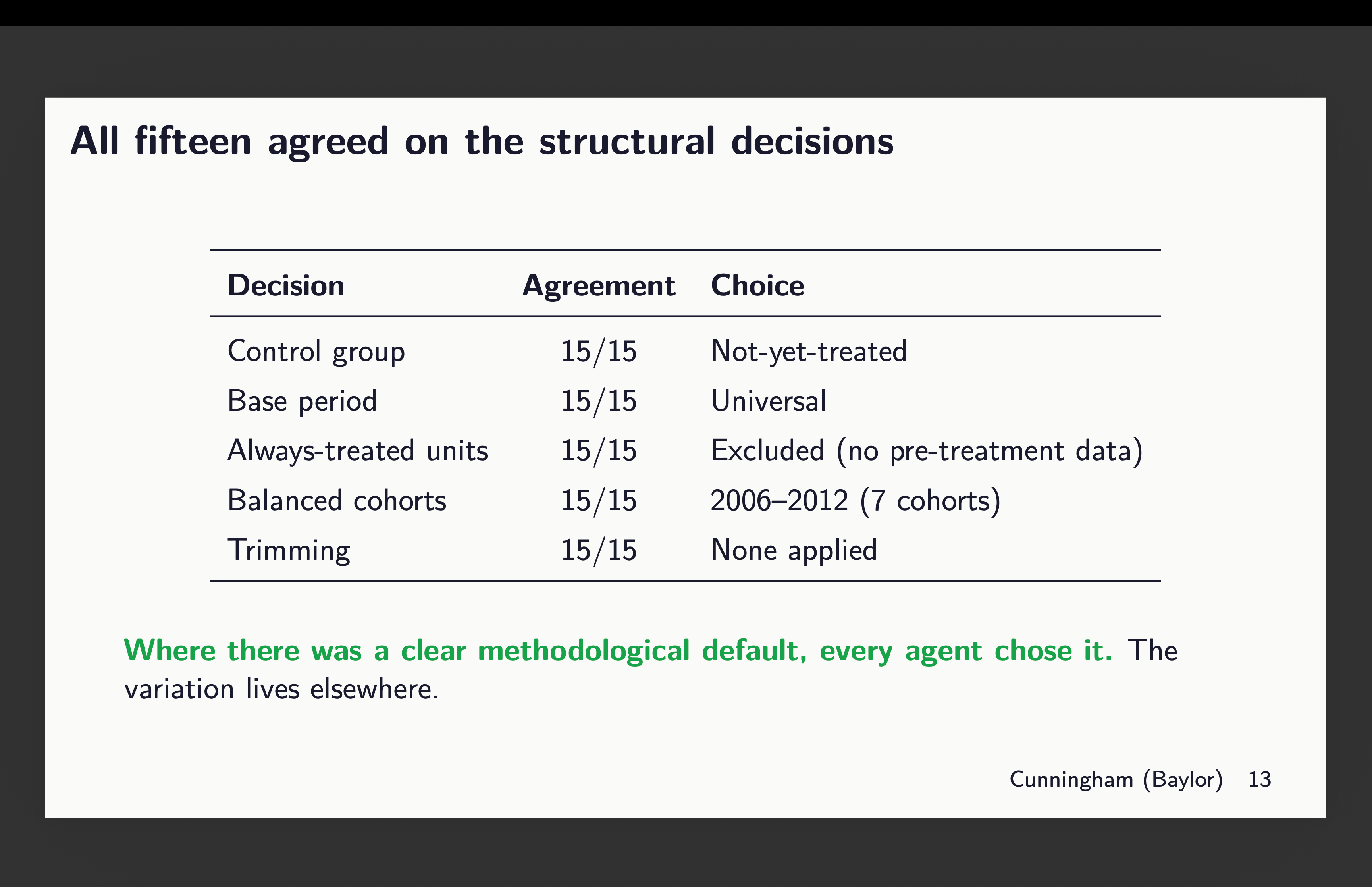
Where there was a clear methodological default — something that follows directly from the instructions or from the estimator’s design — every agent chose it. The variation lives somewhere else entirely.
The variation lives in the covariates
The covariate heatmap tells the story. Log GDP per capita was included by 14 out of 15 agents. Population by 12 out of 15. These were seen as fundamental predictors of both treatment adoption and homicide trends — near-consensus inclusions.
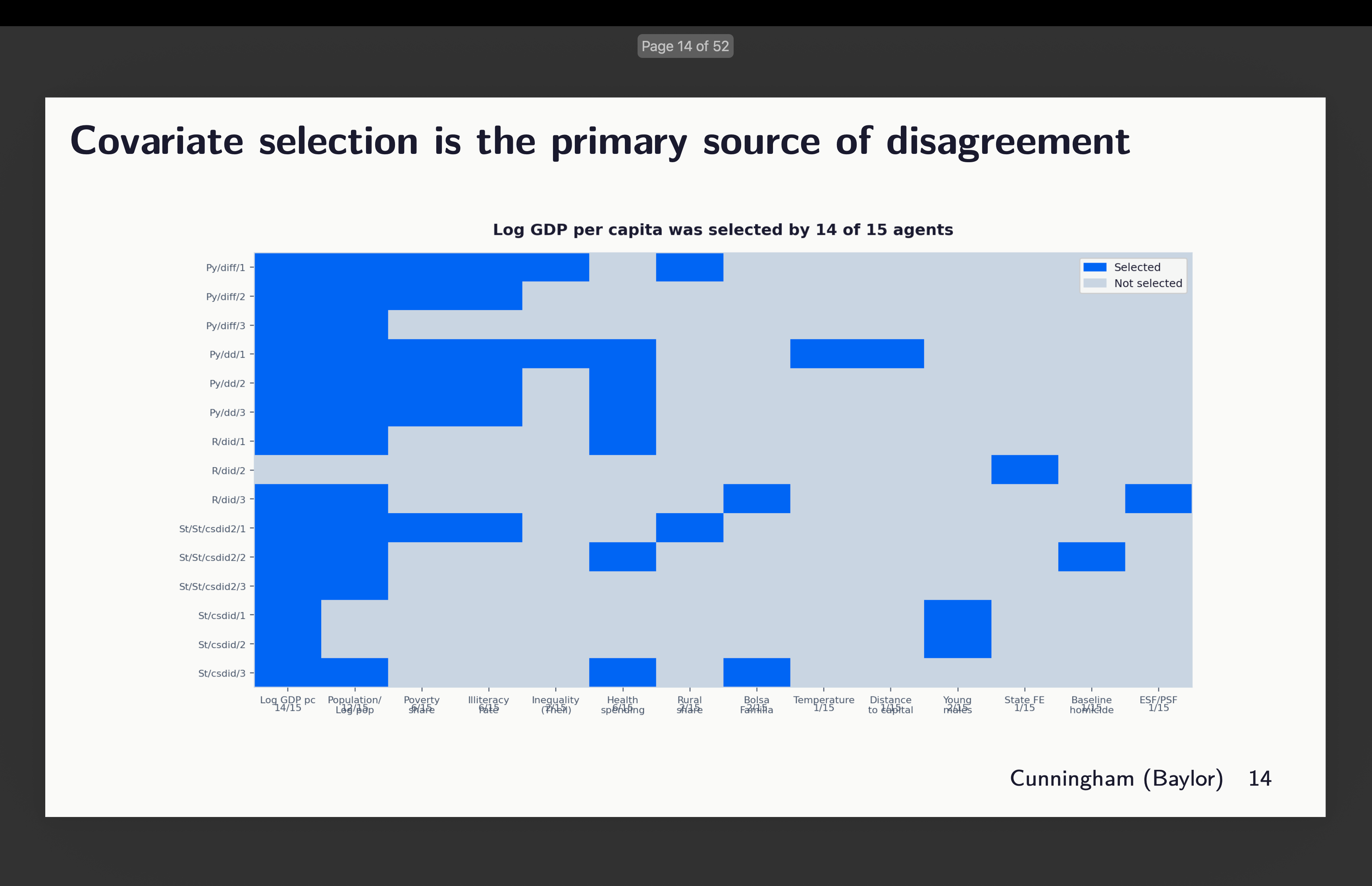
On the other side, geographic variables were rejected by 14 out of 15. Mental health professionals — rejected by all 15 as endogenous to CAPS itself. Health establishments — same, all 15 excluded.
But then there’s the contested middle. Poverty share was included by 10 out of 15. Health spending by 7 out of 15. Bolsa Familia by only 2 out of 15. The agents disagreed on whether these were confounders that needed to be controlled for or potential mediators that would absorb the treatment effect if included.
The reasoning across agents was qualitatively similar — they all talked about endogeneity, collinearity, parsimony. But they drew the line in quantitatively different places. The boundary between “confounder” and “mediator” shifted from agent to agent, and that shifting is where the variation in results comes from.
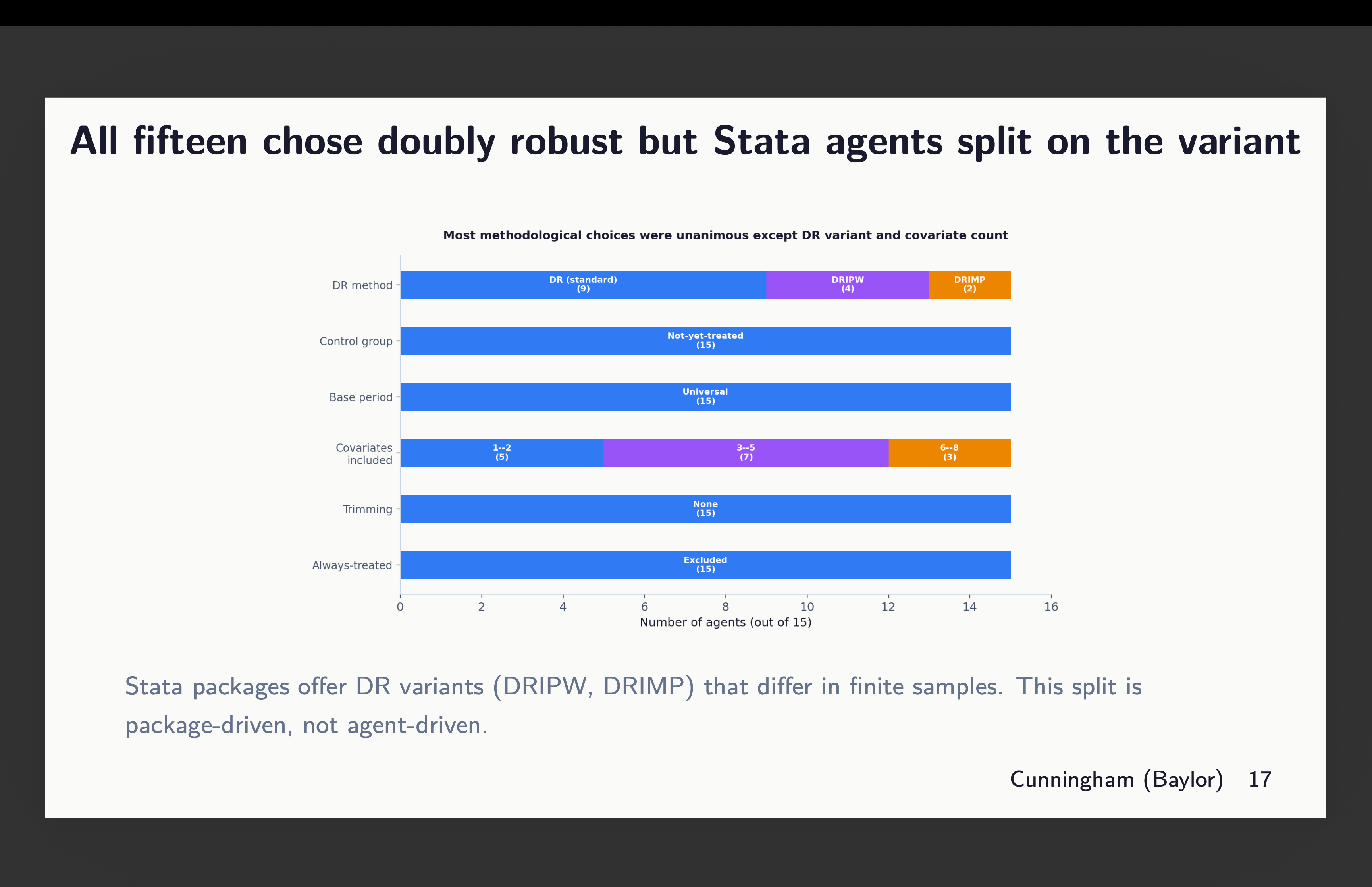
All fifteen chose doubly robust estimation. But the Stata agents split on which DR variant — DRIPW versus DRIMP — and those differ in finite samples. That split is package-driven rather than agent-driven; R and Python don’t expose that choice.
This is where I stopped
The next section of the deck is called “The Event Studies,” and it’s where the actual results start to get interesting — the per-package event study plots, the overlay of all fifteen, a genuine analytical error that two agents made, and the relationship between covariate count and the ATT estimate. After that there’s the anatomy of discretion, the sampling distribution analysis, the comparison to Huntington-Klein’s ratio, and my opinions about each of the five packages.
I’m not going to show you any of that yet.
Partly because I’m trying to keep these walkthroughs shorter. Partly because the setup matters more than people think. The literature framing, the experiment design, the isolation protocol, the covariate heatmap — if you don’t understand why those matter, the event studies are just lines on a graph.
But also because there’s a genuine cliffhanger here. Fifteen agents agreed on everything structural. They disagreed on covariates. The question is: how much does that disagreement matter for the actual estimates? Is the spread tight enough that you’d feel comfortable reporting any single run? Or is it wide enough that the confidence interval from one analysis is basically meaningless?
I know the answer. You’ll see it in Part 2.
So again, thank you for supporting the substack! If you like this stuff, consider becoming a supporter! Here’s a Spotify playlist to help juice the pot.
That cliffhanger is criminal