Claude Code 28: Multiple Agents Auditing Your Callaway and Sant'Anna Diff-in-Diff (Part 3)

Reviewing what we found from our run

Last week I had Claude implement a “multi-analyst design” across 5 Callaway and Sant’Anna packages (2 in python, 1 in R, 2 in Stata) on a fixed dataset, a universal baseline, ~20 covariates to choose from for satisfying conditional parallel trends, and the same target parameter. You can find that here:

But in that post, I didn’t finish reporting it. So I filmed myself going through the “beautiful deck” it produced. And in this substack, I’ll explain in words what it found, but the gist is that there was surprisingly large amount of variation between packages but also within packages in the variation in the results across 15 total runs. Here’s the video:

And I just wanted to again thank everyone for supporting the substack. It has been really nice to write about Claude Code these last two and a half months since my first post December 13th, 2025. I’ve been learning a lot over these 28 posts (!). I really enjoy trying to figure out how to use Claude Code for “practical empirical research” — everyday, run of the mill, type of applied stuff. And it’s been a bit like trying to ride a wild stallion. So that’s been fun too as I needed the excitement.

If you are a paying subscriber — thank you. I appreciate your support. And if you aren’t a paying subscriber, remember that the Claude Code posts are all free for around 4 days, but then they go behind the paywall. The more typical non-AI posts are usually randomized behind the paywall, but as Claude Code is a new thing, and I want to help people see its value for practical empirical work, I post those for free, they sit open for four days, and then they all go behind the paywall. Hopefully that’ll be enough to help you see what’s going on. But perhaps this is the day you feel like becoming a paying subscriber! At only $5/mo, it’s a deal!

---

Breaking down what I found

So if you go back to that previous entry (part 2 specifically), you will get the breakdown of what this experiment is about. And if you want to watch the video, that’ll help too. But let’s now dig in. You can also review the “beautiful deck” too if you want.

There’s two “target parameters” in this exercise of note. The first are event studies which aggregate up to all relative time periods and if cohorts differ in size, and the weights are proportional to cohort size, then it’s a weighted average using cohort size as weighting at the appropriate places. I also am balancing the event studies which means the same cohorts appear in all l=-4 to l=+4 relative time periods. Therefore no compositional change in who is and is not in each of these event study plots.

So that’s one of the parameters. And the other is I’ll then take a simple weighted average over l=0 to l=+4 (thus each weight there is 0.2 off an already weighted average that used cohort size as weights for the event studies). And therefore in these, we’ll see both.

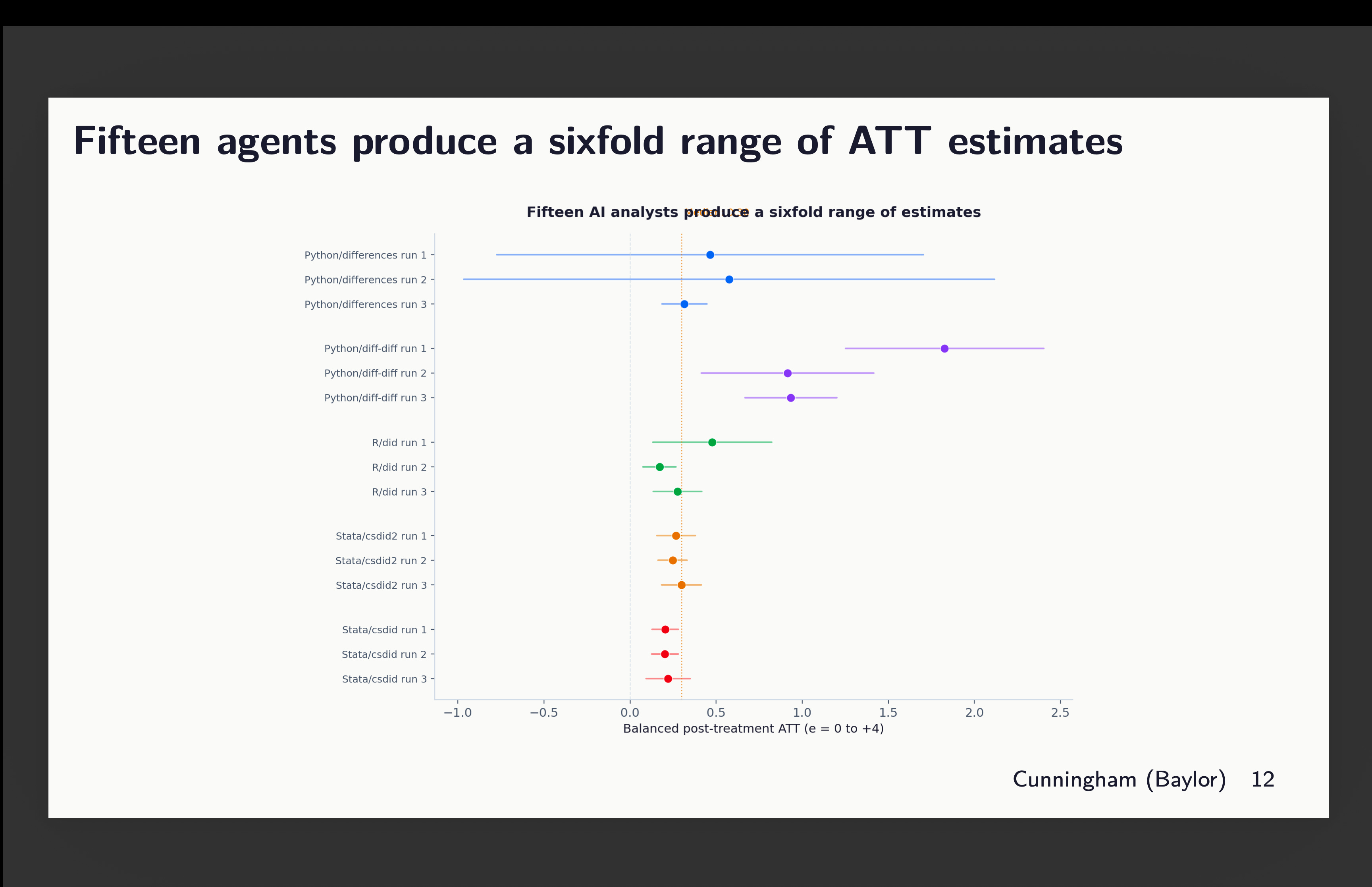
Forest plot of average point estimates

The first though is a forest plot of the 15 estimates across all 5 language-packages. And this is pretty interesting because notice that while all of them are positive effects, 2 of them have huge confidence intervals, and one of them (python’s diff-diff run 1) is large and statistically different, not just from zero, but from 11 of the others. The rest are around 0.4 on average.

Event studies

Here are the individual point estimates from the event studies all laid on top of each other:

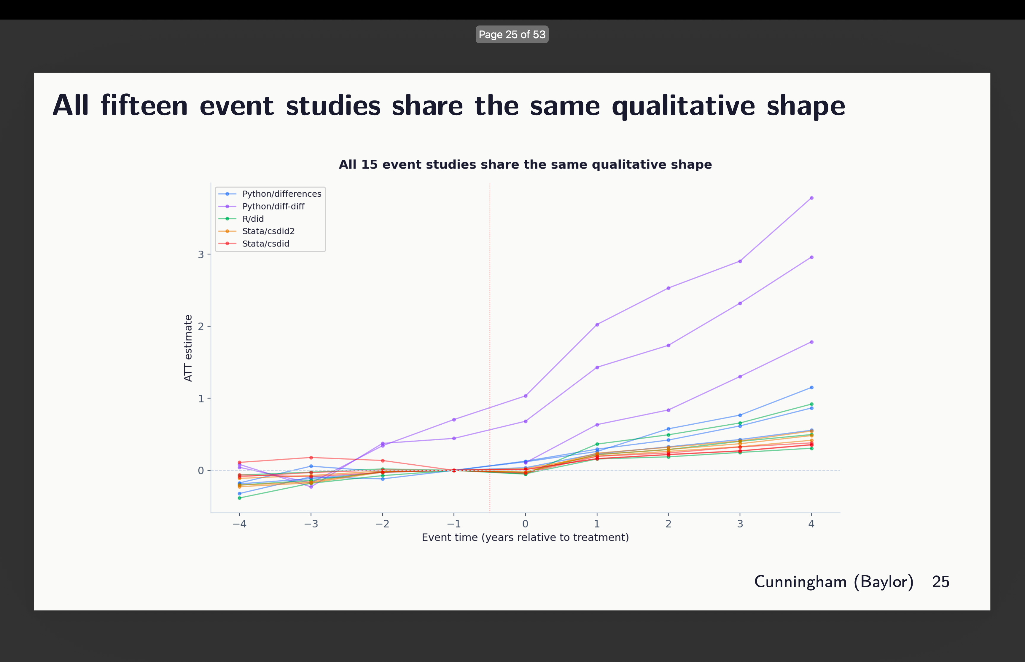
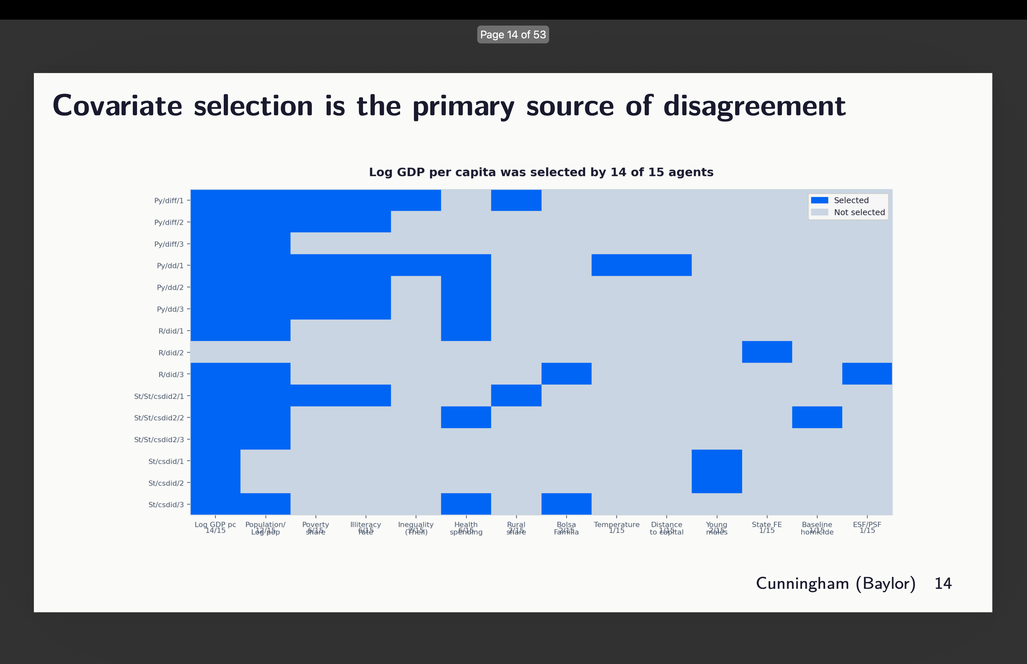
So you can see here some odd things. First, it appears that two of our runs did not obey orders to use the universal baseline. Notice that there are two graphs rising from around l=-3. That’s the python package diff-diff. I’ll show you that in a second. The others are similar-ish, but they bear looking at more closely. I’ll discuss them in order. But before I do, let’s just remind ourselves which runs chose which covariates with this graphic:

Python’s differences packages

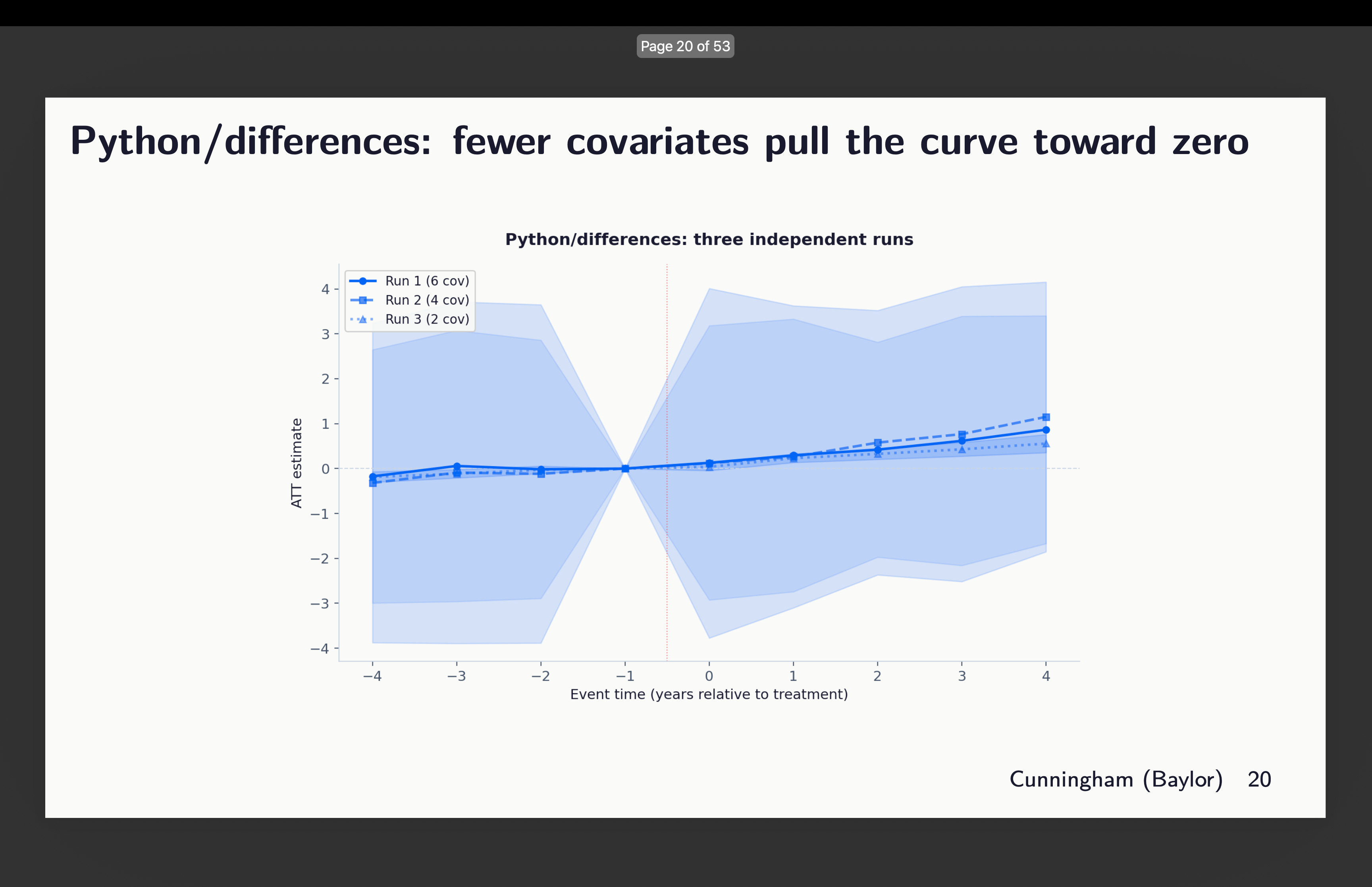
First I looked at the three runs from differences written in python. Now here’s a strange thing though — why are these 95% confidence intervals massive? Look how they range pretty much from -4 to +4. Why is that? So that’s something I want to better understand, but for now notice just that they do, and that the differences within this are covariates of 2, 4 and 6 chosen. You can see above which ones that was.

Python’s diff-diff

Next is Isaac Gerberg’s ambitious diff-diff package which he has been building all this year. What did we find there? You can review the covariates chosen above to interpret these results.

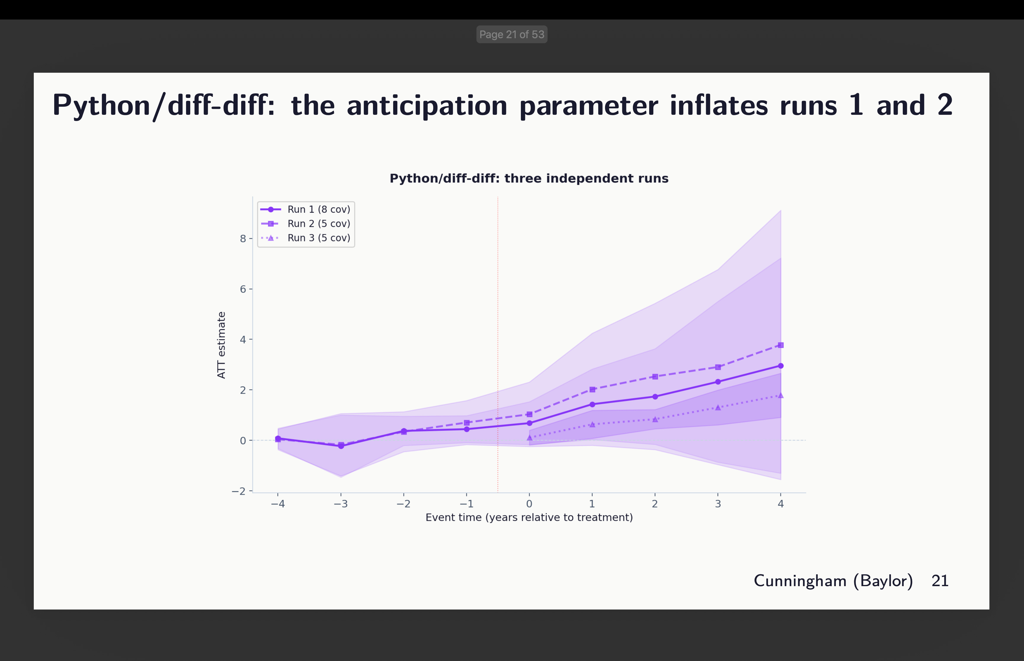
Okay, well this is a strange one. Why? Because Claude literally refused to do what I said here which was use g-1 as the universal baseline. In two of them, it used g-5 as the baseline. And in one of them, it did use g-1, but did not estimate the pre-treatment coefficients.

This is a good place to just pause and say something about using g-5 as your baseline. That’s absolutely find to do. But note that when you do it, while your target parameter stays the same — we are in each of these estimating aggregated ATT(g,l) parameters — the parallel trends assumption is changing. And that is because in Callaway and Sant’Anna, treatment effects are estimated using whichever baseline you pick and are always “long differences” too. The pre-treatment coefficients can be either long or short differences, but the treatment effects can only be long differences. Which means the parallel trends assumption is always long differences too. In fact when in doubt, just remember that in CS, whatever is the description of the characteristics of your ATT(g,t) target parameter (e.g., covariates, weights) carries over to your parallel trends assumption too, only it is then a diff-in-diff simple 2x2 estimated as long differences in the potential outcome, Y(0), itself.

Which is to say that while the target parameters are the same here, the parallel trends assumption is shifting around. And that’s find if you have balanced pre-trends, but here we don’t, which is itself interesting, and that as a consequence the python differences packages is finding much larger coefficients in post and pre than others do. It does not appear to be an error so much as Claude didn’t understand the documentation and couldn’t therefore figure out how to implement what I asked. This is something I’m working on next.

Original R did

Next I looked at the event study plots for R’s did. And this one again chose different sets of covariates, but here’s what worrying — the one that chose 3 (out of 21 covariates mind you) shows signs of trends, whereas the one with only 1 covariate looks flatter. So which is it? Which of those three do you think satisfies conditional parallel trends?

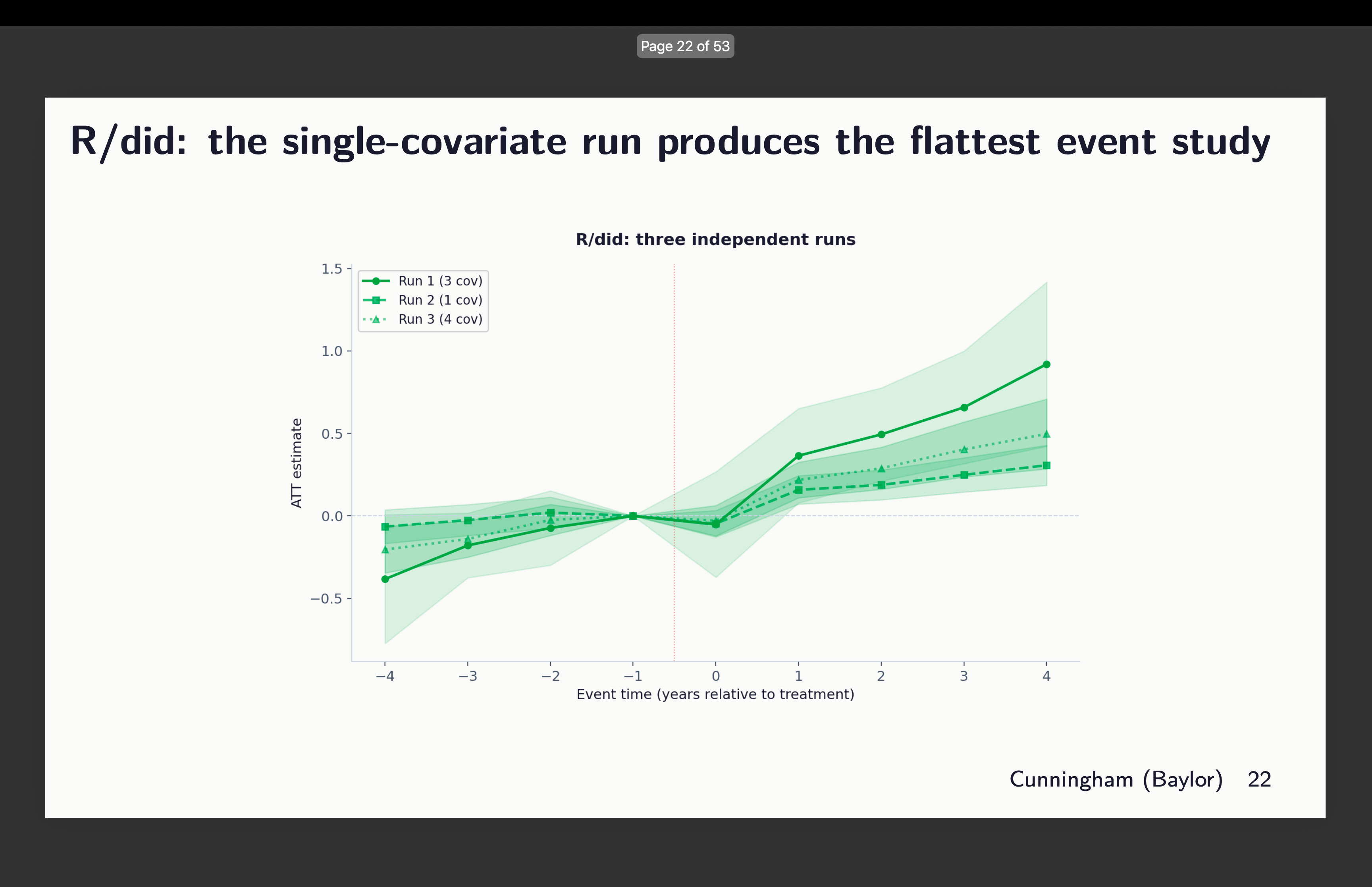
Think about it for a moment. How many papers have you ever seen that shows variation in estimates across covariate selection and package selection? How about none? What do you typically see instead? You more often see robustness to which diff-in-diff estimator — the famous “all the diff-in-diff plotted on top of each other” graphic. But you don’t ever see someone exploring covariates or packages. Moving on.

Stata: csdid2 and csdid

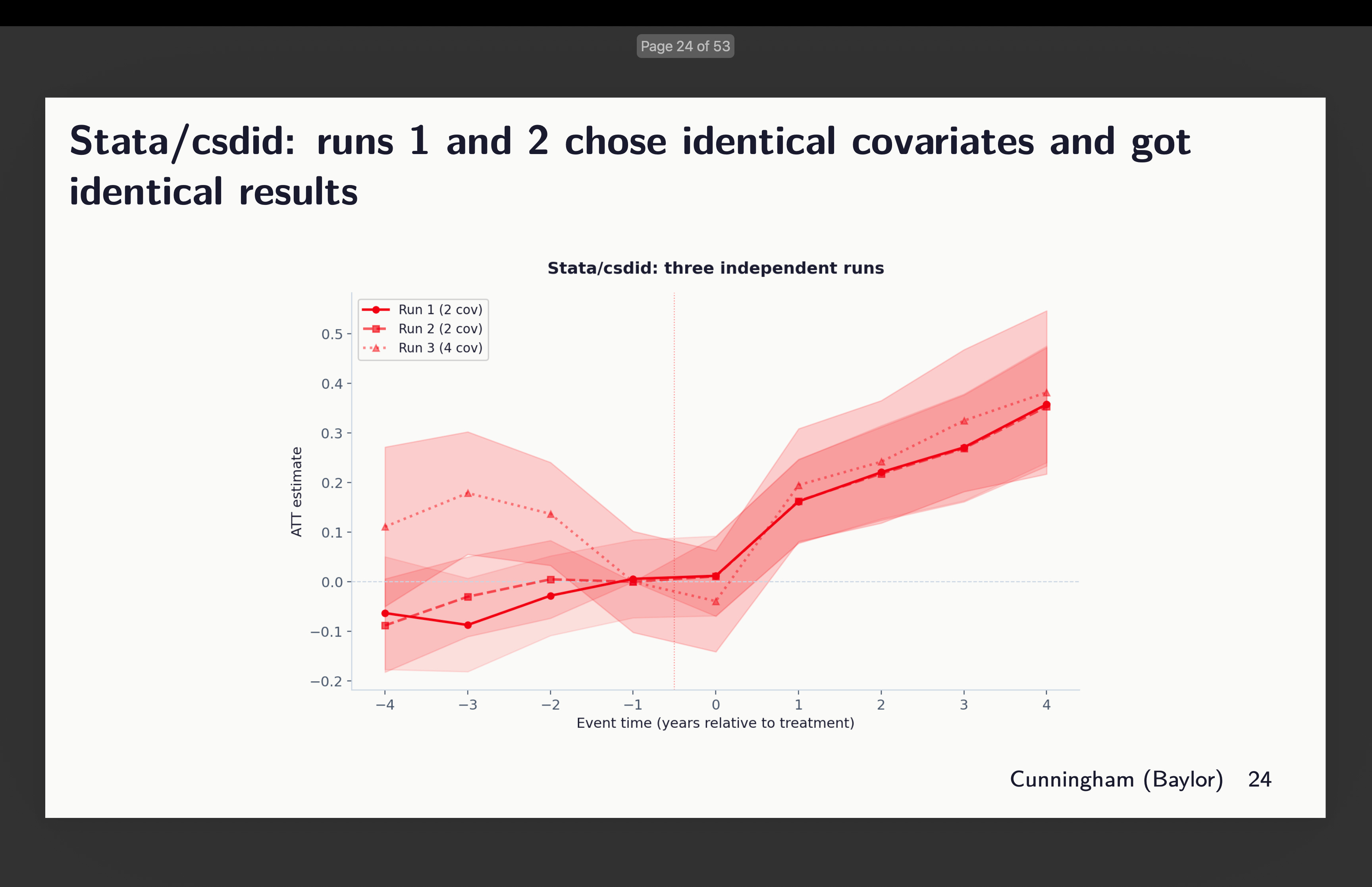
And finally, I look at the two Stata packages: the commonly used csdid (available from ssc) and csdid2 (now archived). I included it because Claude chose it, so I included it because I think people may want to use it as it’s fast. Though in our case it was not as fast as R. There’s not a lot to report except to say that depending on which and how many covariates to condition on, we might see signs of rising trends — some more worrisome than others

And then I looked at csdid. Claude said they chose identical covariates. But it’t not clear to me then why pre-trends are different. I didn’t dig into this because I’m rerunning the whole thing now with 20 agents per package (and one more additional one) to get 120 estimates, and then I’ll dig into that. But here’s that event study.

Variation Within and Across Packages

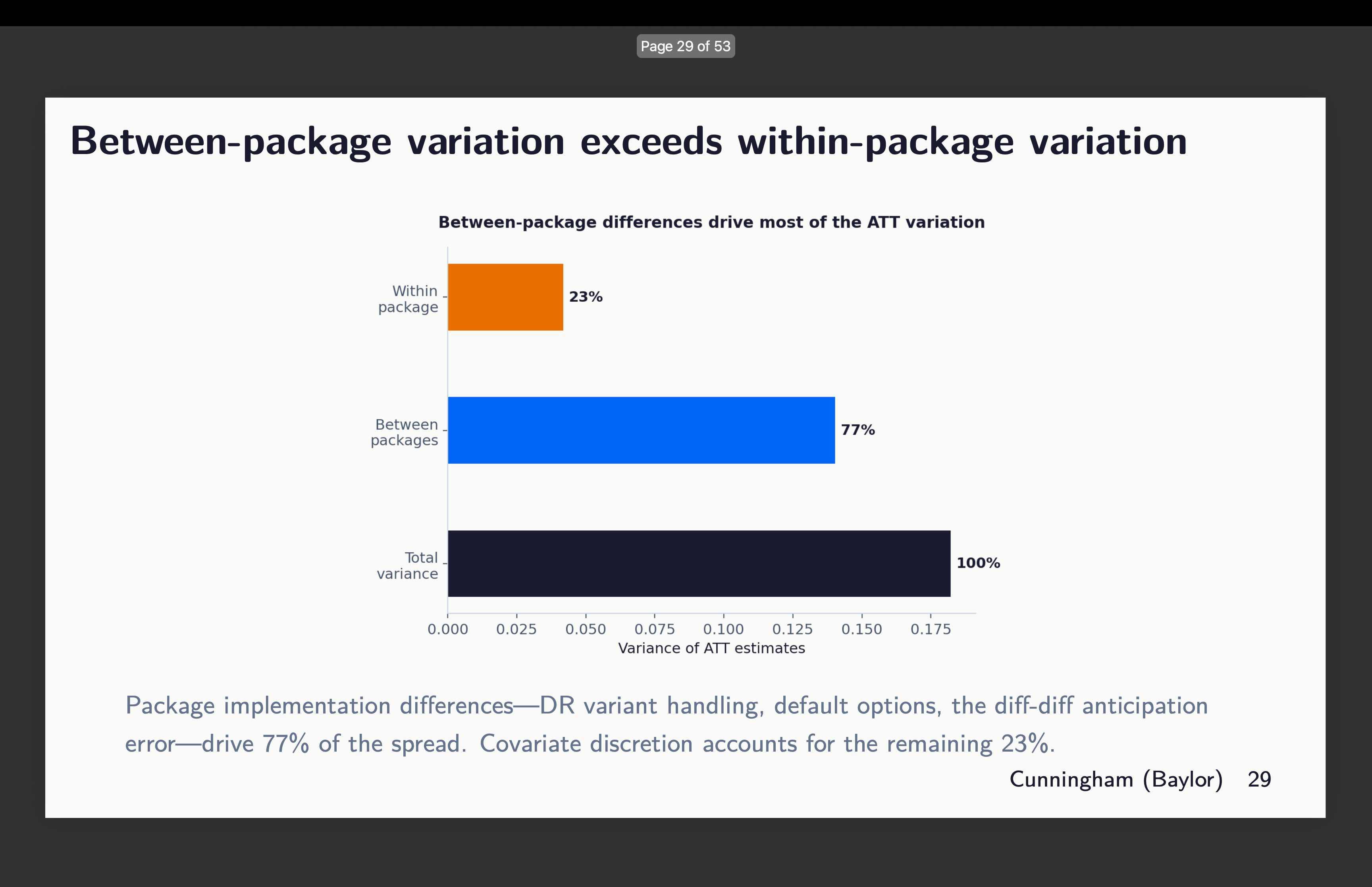
Okay, so now this is the weird result. The more covariates included, the larger the point estimates altogether. You can see that here, but notice that most of this is coming from the variation across packages which you can see if you look closely at the colors. That big outlier at the far right is actually the python diff-diff one that used both 8 covariates (hence why it’s up there), but also used g-5 as its baseline. And remember because of slight rising trends in the pre-period, by the time it gets to the end of the periods, it’s got a head start and is rising. That’s why it’s averaging out to 1.75.

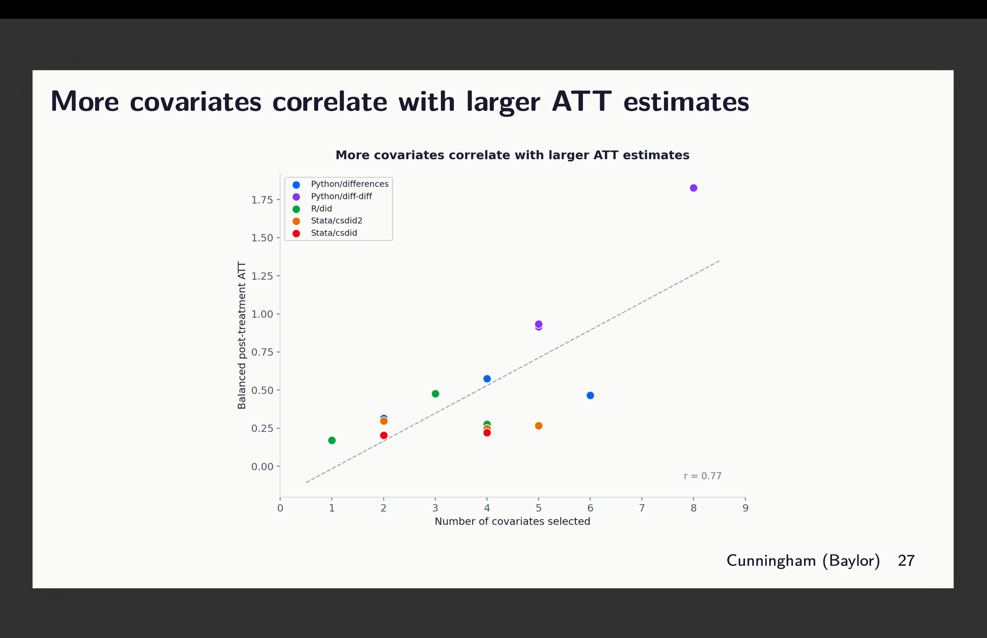
But even throwing out that outlier, you can see still the correlation — the more covariates included, the larger the ATT estimate we find, even though all of these agents use the same dataset, method, baseline, estimator and double robust, given only the instructions to “choose covariates that satisfy parallel trends”. So simply by picking more or less covariates, you get larger or smaller effects alone.

But then the other dimension where there is a lot of variation is the between packages. There is variation within too, but around 77% of it comes from the selection of which software package to use. See here:

Supporting Reasons

Now I want you to think back to the last time you saw a talk using diff-in-diff when the researcher listed covariates. Did they spend more time explaining the estimator or did they spend more time explaining the covariates and the rationale for each one of them? And did they ever mention which package they used? I bet good money that talked more about the CS estimator and the assumptions than they did covariates or package, and probably did not mention the package because why would they? Aren’t all the packages giving the same thing?

So I don’t know yet the answer to the last thing because in no single case did any two agents use the same covariates across packages. So that is still something I’ll look into but it’s not here because this is not about software robustness; it’s about discretion on a single dimension — covariate selection. And I bet you rarely have you heard someone spend as much time explaining what and why those chose covariates as they did talk about the actual econometrics, right? The agents were instructed to explain their rationale and here it was:5

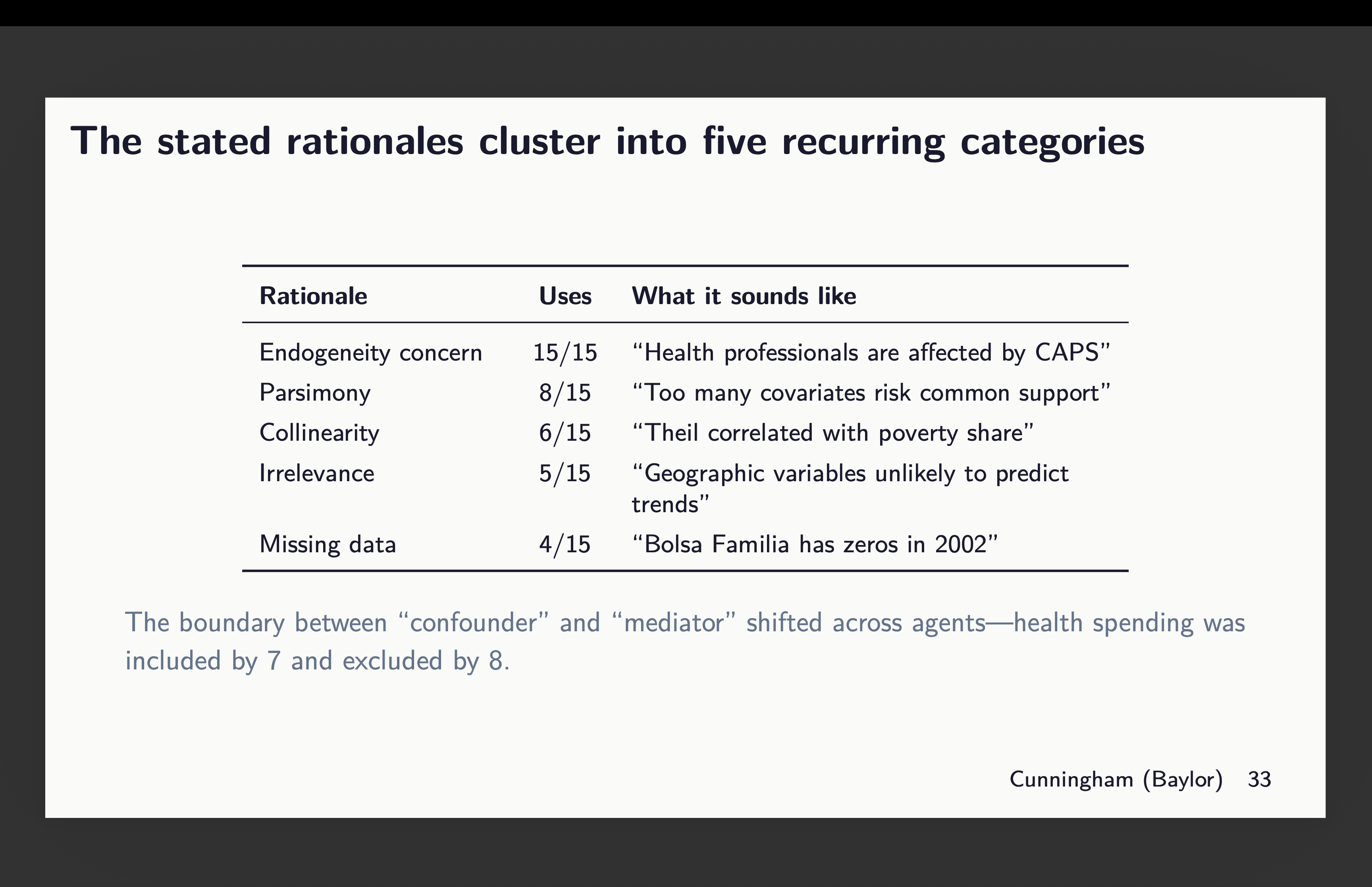
There’s basically reasons they gave for covariate selection and they’re listed above. Now I want you to imagine for a minute you’re in a talk, and someone does explain their choice. Would you object to their explanation? Probably not. You’re more likely to object to the estimator (“why are you using TWFE?”) than you are to the covariates, and yet covariates are driving variation in estimates in this experiment. So just let that sink in.

How big of a difference? One of them R agents using did chose only state fixed effects (remember this is municipality data so there is variation within a state fixed effect for estimating that first stage). For it, the point estimate was 0.17.

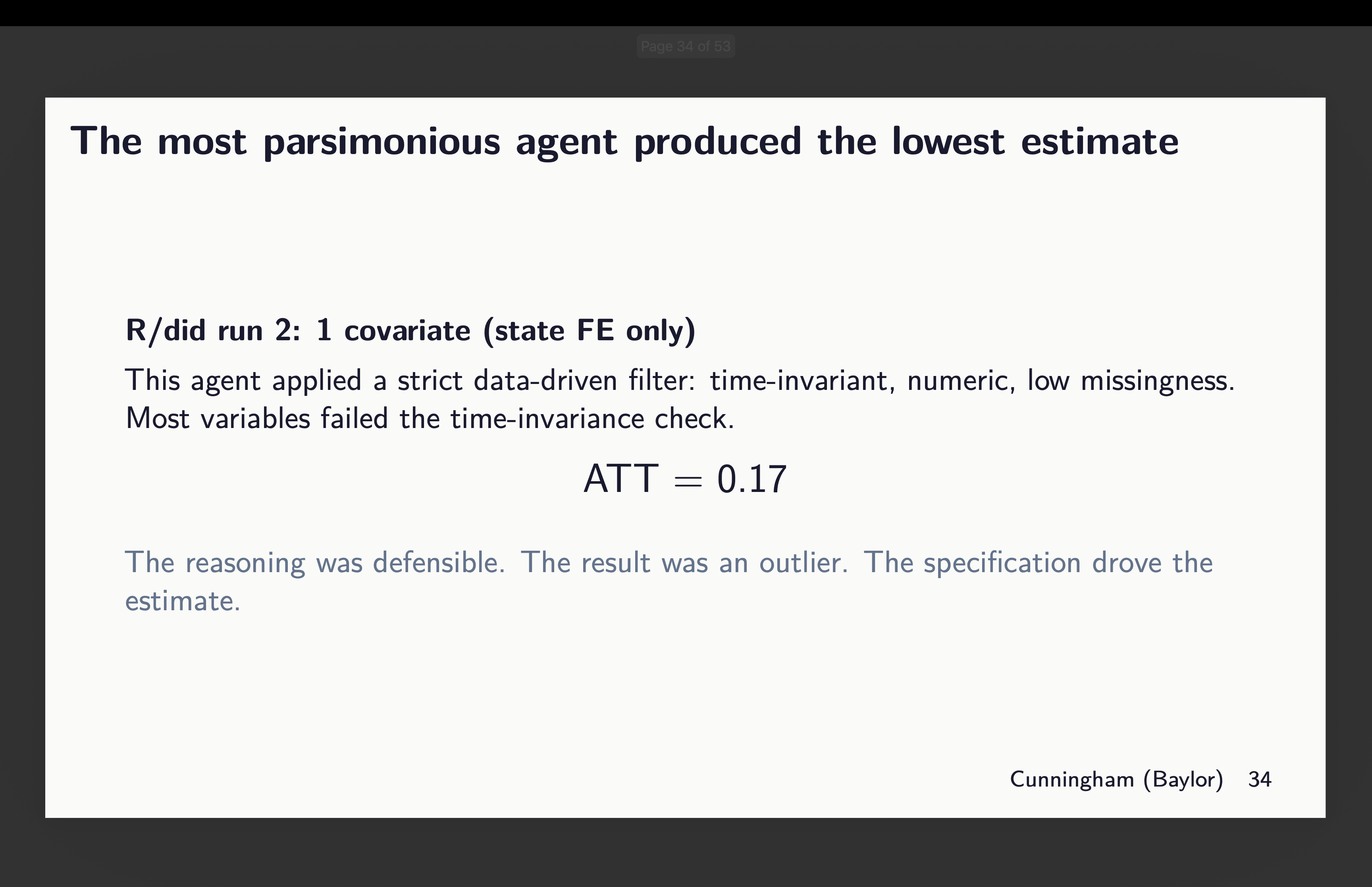
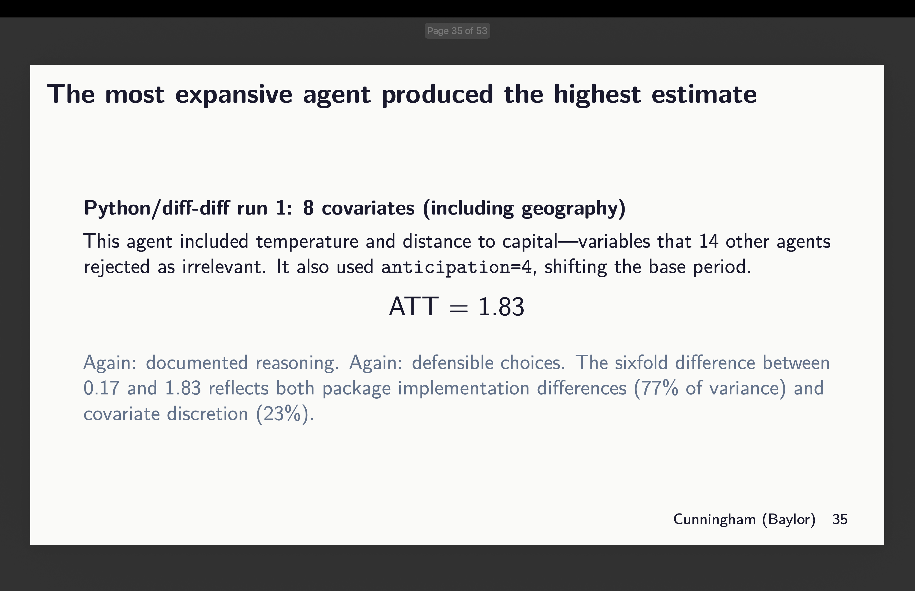
But now look at the agent given python’s diff-diff who chose 8 covariates. Its estimate is almost 11 times larger. And both documented their reasons, and arguably all of them were defensible. I don’t know why Claude said this is a six fold increase when 1.83/0.17=10.765 but whatever.

How big are the “non-standard errors”?

Now to the best part. Given we have 15 estimates, aggregated into that simple ATT, weighted over all post-treatment ATT(g,l) from 0 to 4, what can we do to measure the uncertainty in this parameter. Let’s pause for a second and review what the standard error means in the first place.

Under repeated sampling, you get a series of hypothetical samples from which you’d run CS on each one, and then when you look at the distribution of those estimates, you have a random variable that varies according to that models application to its own i.i.d. drawn sample. And the standard deviation in that sampling distribution is what our standard errors are meant to capture. In the normal distribution, 95% of probability as a single unit is within approximately 2 standard deviations from the mean. And thus the p-value is based on the sampling distribution of the t-statistic - what percent of t-statistics are more than 1.96?

Okay, but then what about if we have a fixed sample, fixed dataset, but only allow for discretion in covariate selection and package? And we allow n to be 15, with 3 runs per package? Well that is not what our standard errors are meant to capture even though that will have a distribution. And if it has a distribution, it has variance, mean and standard deviation. But I also have the standard error for each run, as well as the point estimate.

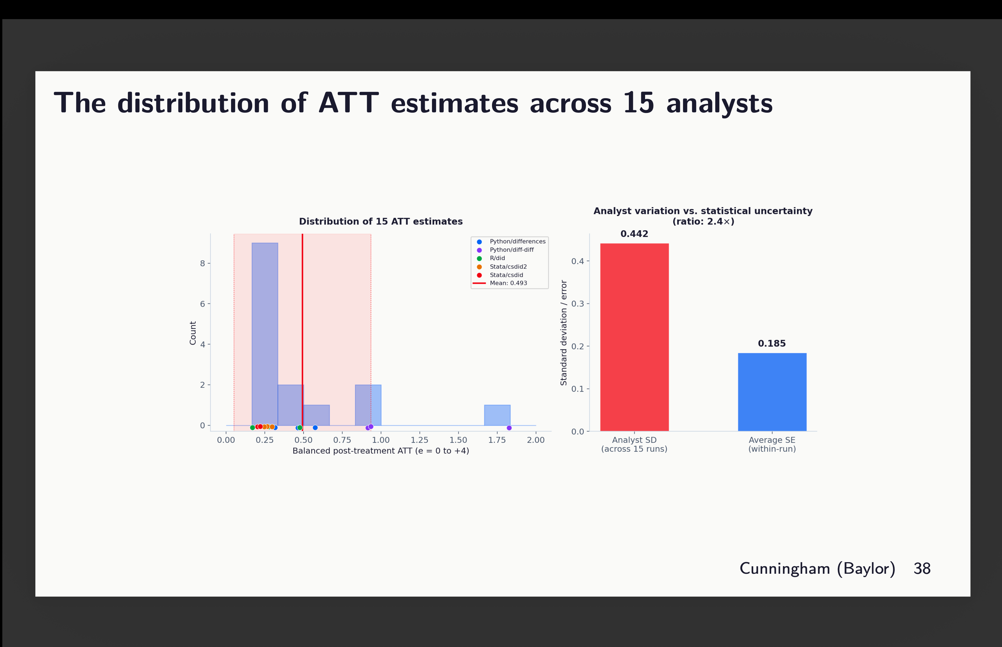
So what we have here is just that but summarized. And check this out. The red box on the right is standard deviation across all my point estimates (including the outlier from python diff-diff). And it’s a 0.442 standard deviation. But if I took the average of all 15 standard errors, that is 0.185. And thus we get a 2.4 times larger standard deviation in our 15 estimates than the average standard error for those 15 estimates.

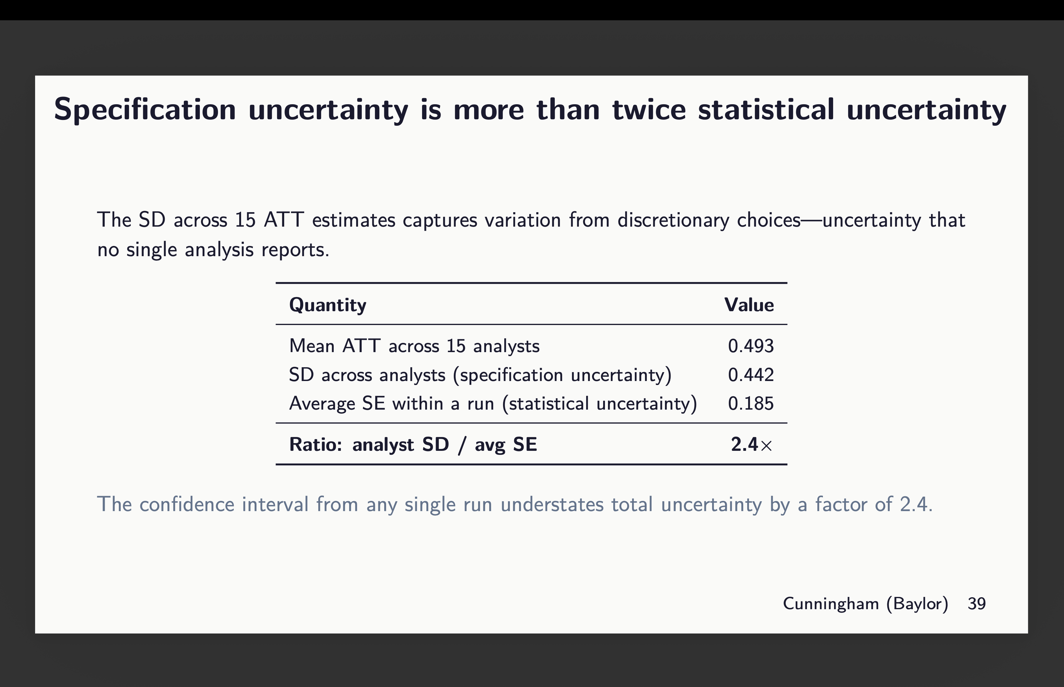
So now let that sink in. The standard errors we report are based on repeated sampling. They are designed to measure the statistical uncertainty associated with the sample and its correspondence to the population parameter. They are not meant to measure uncertainty in which team worked on the project. And yet there is that because each team is picking a different covariate combination even with the same dataset and even with the same estimator and even with the same experimental design.

So what’s next?

So next on the menu is a few things. They are:

1. I’ll add in the doubleml package. It’s different architecture, but it’s a reasonable one to use. But otherwise it’s all five of the ones I reviewed here plus a sixth.

2. I’ll increase the runs from 3 to 20 agents per package giving me 120 estimates when it’s done.

3. I’ll continue to use CS in all of these with the exception that doubleml will be different in its own implementation, but that aside. Same donor pool of covariates, same not-yet-treated comparison group, same universal baseline (hopefully fixed this time for python’s diff-diff), etc.

4. But now I am going to allow for any covariates ranging from none to all and any combination it wants. The only rule is “choose what satisfies conditional parallel trends”.

5. Each run will compute the standardized difference in means on covariates using baseline values averaged. It’s not ideal, but whatever — I need this to not go on for a million years.

6. And each will now have the option to use IPW, regression adjustment or double robust, and if Stata, then whichever DR it wants.

So I’m just going to be carefully documenting this all and maybe at the end of this, I’ll have learned something, and if so, hopefully all of us will learn something. But I am becoming more and more of the opinion that we need to be documenting this package and covariate selection a lot more carefully than we are. Packages all use the same assumptions and are supposed to be identifying the same parameters. Their differences should be things like speed and efficiency in the CPU. It should not be actual differences in numbers calculated. Standard errors will be different due to bootstrapping which uses random seeds, but the point estimates should be the same given the same covariates and modeling of those covariates in the first stage.

But the covariate selection and how those are modeled — that is the other two things I’m trying to pin down. So let’s see what we find. I will have text by each agent explaining their reasons and I may send all 120 of those reasons to openai to have gpt-4o-mini classify them. That may be overkill, but I love doing that and so may do it again.

That’s it! Stay tuned!