Covariates, diff in diff and Lalonde test

Well can you believe it? I caught Covid. There’s a strain going around Boston and I drew the short straw. Forgot how pleasant this was — pounding headaches, eyes that feel like they’re burning from the inside out, congestion and scratchy throat, and fever. So what better thing to do than write a substack about Lalonde and diff in diff and covariates. So here’s the test.¹

Lalonde famously showed that many econometric evaluators were biased, in their application not in their properties and estimators. An estimator can be unbiased and yet be misapplied and thus biased. And he showed cleverly that that was the case in his 1986 job market paper.

He took an RCT, first, and compared 1978 earnings for a treated and control group. That difference was $800. Meaning that the treatment — a job training program aimed at poor workers — raised the real earnings of workers by $800.

Then to show the problem facing the current econometric evaluators, he dropped the control group — which was recall exchangeable with the treatment groups counterfactual earnings due to the randomization — and replaced it with that of survey data of Americans, notably the CPS and the PSID. He then used a gamut of econometric estimators to estimate the effect of the program which was still, expressed as an ATT, $800. And his estimates did not recover it. In fact estimates ranged from -16,000 to +3,000 and the few that got close did not have any obvious ex ante reason to favor them.

And thus the credibility revolution was born.

---

I want to do the same thing, only I want to make three changes.

1. I want to use the Dehejia and Wahba (2002) sample which is a subset of the workers who had two years pre treatment earnings available. The effect there is higher — $1,794. That’ll be our target.

2. We will use difference in differences with the CPS sample for our non random comparison group. The target parameter there is the ATT and the effect is still $1,794 because the ATT is the effect on the treated workers, and the treated workers remained in the sample (just not the original control workers). This is a subtle point maybe but it’s worth saying — the ATE and the ATT had been under randomization $1,794 because under randomizing, they are the same. But the ATE changes when we replace the experimental control with the non experimental control group — it’s just the ATT does not.

3. We will use covariates with the diff in diff estimators but under different specifications, including the two way fixed effects model with additive covariates which is the most common probably of all applied panel estimators.

---

I’m going to review six estimators, all diff-in-diff. And remember — the effect is $1,794. It’s known. It’s the ground truth. So we judge performance against it. And my contention in this is to show you that a) covariates can matter a lot, even with diff in diff and b) that does not therefore mean that all ways of introducing Covariates into a diff in diff model are equal.

Recall from our JEL that there are four separate regressions that are numerically the same for calculating the estimated OLS coefficient. They are saturated dummies where you have a treatment dummy, a post dummy and an interaction. The interaction is the numerical equivalent of calculating four averages and three subtractions. Then there is the inclusion of worker and year fixed effects with an interaction of post and treatment. Same exact calculation on the interaction. Then there is a first difference regression onto a treatment dummy. Same thing. And then there is an across-comparison group regression onto a post dummy.

1. Interaction OLS without covariates

Since they are all the same we use the one that will let me later include time invariant covariates: the saturated regression. And when we do this, we get $3,621. This is positive but it’s two times too large.

2. Interaction OLS with additive (but not saturated) covariates

Next we run the typical diff in diff of simply including covariates additively. This also yields $3,621. Note that I did not use TWFE, which would have eliminated the time invariant variables entirely through the demeaning process, but as the TWFE and the interaction of all dummies is the same numerically, it doesn’t matter. When we do this, we get this 3,621.

But notice that it is the same number. Why? This is because they do not change over time. Since the TWFE and saturated regression are numerically identical, then even when TWFE deletes the time invariant covariates via worker fixed effects, the actual did coefficient is unchanged because the estimate never depended on them anyway.

3. Regression adjustment I: interact the covariates with time

The first adjustment we will consider will address the problem of a misspecified regression in which covariate trends do not change over time. What is this though?

Let’s say in our sample there’s two types of workers for simplicity. Those with a high school degree, and those without. Covariates trends asks if the high school educated workers are on different Y(0) trends than the ones that don’t. If they are, then the above regression I did is incorrect insofar as the treatment group has more of one than the other. And it does — our control group is from the CPS, a representative sample of America. The average American had more schooling than the individuals in the MDRC job training program. So, if we think their trends are different, then the imbalance in schooling will violate the parallel trends bias term.

Conditional parallel trends will fail due to the imbalance but we can correct at least part of it with partial saturation, which is to interact the year dummies with all the covariates.

When we interact all the covariates that Dehejia and Wahba use, interestingly our estimate drops to $1,711, which is almost exactly the true ATT of $1,794. This suggests that covariate imbalance is a nontrivial problem with these data and that if the groups with different covariate combinations are on different earnings trends, Delta Y(0), then the imbalance breaks conditional parallel trends mechanically. You have to interact with X to fix it, not simply include them additively, because you need to model those trends explicitly first.

4. Regression adjustment II: heterogenous treatment effects and saturated regression

But imbalance is only potentially part of the problem with specification #2. It also imposes constant treatment effects with respect to the covariates themselves. Using our schooling example, but allowing schooling to enter in additively, the treatment effects are the same for high school and no high school educated workers.

We correct this through saturation which is to dummy out every value of the covariates, interact it with the treatment, and run that regression. Then you recover the ATT by summing over all the treatment indicator coefficients (both it alone and the interactions) multiplied the same mean of the covariate in the treatment group.

Interestingly, this did nothing to our estimates. We find using this form of interaction the same as what we found using the additive method — $3,621. Why? Because saturating on a regression involving levels did nothing to address the conditional parallel trends assumption, which is in trends, not levels. Until we do that, we are going to continue to suffer from a violation of conditional parallel trends.

5. Regression adjustment III: saturated in time and covariates

So, now we will do both. That is, we will interact time with the covariates, as well as interact covariates with the treatment. And then we will recover the ATT by summing the treatment coefficients (including the interactions) times the sample mean of the covariates in the treatment group only. In diff-in-diff, this is often called outcome regression, based on Heckman, Ichimura and Todd (1997, Restud). But here I do it manually, and to do it manually, I first take first differences in earnings, then I regress that onto the treatment dummy, each covariate on its own, and the treatment interacted with each covariate. There’s no post dummy here though. The first-differencing removed it.

Here’s the subtle part: because the outcome is now a change, a covariate’s own coefficient is no longer a level effect. Rather, it’s the covariate’s effect on the trend. That main effect is the X-by-time interaction from #3, for free. So the first-difference regression does two jobs at once: the covariate main effects bend the control group’s counterfactual trend (what #3 did), and the treatment interactions relax constant treatment effects (what #4 tried to do). That’s why it lands at $1,770 while the pure-levels version in #4 sat at $3,621. Because the levels saturation never touched the trend and thus the imbalance became problematic.

6. Heckman, Ichimura and Todd (1997)

But guess what. The Heckman, Ichimura and Todd (1997) estimator which moves in a few stages is the same as the regression adjustment “both” we just did. The stages are:

• Regress the first difference, Delta Y, onto X for control group only

• Collect the coefficients on X, transport them to a regression model aimed at the treatment group only, and predict Delta Y for the treatment groups only

• Calculate individual treatment effects as the treatment group first difference minus the imputed counterfactual first difference for the treatment group only and then take its average over the treatment group.

That’s what I find so interesting and not terribly intuitive. That when you do that fully interacted X on a first difference regression for all units (treatment and control), it is numerically the same as if you had gone through a series of steps starting with the control group only, then predicting on the treatment group only. This is, though, what the Oaxaca-Blinder estimator had done which is itself too a treatment effect estimator for the ATT, the ATE and the ATU depending on how you want to go about using those interactions. Nonetheless, doing this we get $1,770.

7. Propensity scores and double robust

I can also introduce the covariates via an inverted propensity scores reweighting procedure developed by Alberto Abadie (2005, Restud), or I can introduce both regression adjustment and the propensity scores reweighting procedure in what’s called double robust developed by Sant’Anna and Zhao (2020). I’ll explain these two later, but for now I’ll just show it to you, and the code will be below at the end of this substack.

---

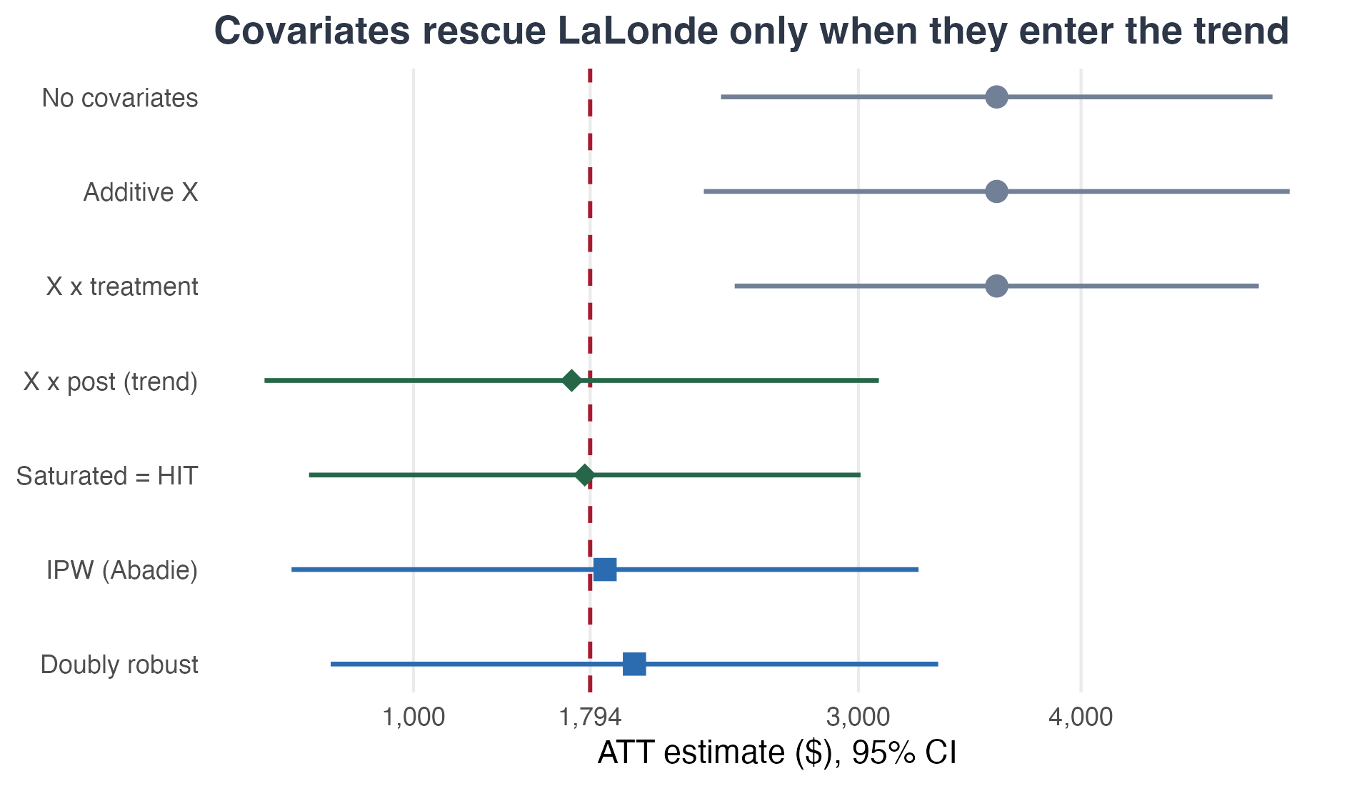
So let’s summarize this. First of all, the Lalonde data is the gift that keeps on giving. We know the ATT is $1,794, and we therefore can convincingly show (in my opinion anyway) that the exclusion of covariates in a diff-in-diff can be the wrong spec. Furthermore, just because including covariates in diff in diff changed the coefficients does not mean the original was wrong, because covariates are not a robustness exercise. If they were robustness exercise then yes — we’d expect them to not matter. But if covariates perform an actual function, which is satisfying conditional parallel trends and relaxing constant treatment effects assumption, then naturally they both will matter under imbalance and heterogenous treatment effects and should be included.

But that’s the second point I want to leave you with. Just because they are needed does not therefore mean that any specification is equal. As we saw here, the most flexible ones recovered the true ATT or got very close, but the TWFE one even with covariates did not.

---

There’s more to this than I cover here — like why use regression adjustment? Why not use the propensity score method that Abadie developed? What exactly makes them different from one another? What exactly makes one more appealing than another? That’s for a different day. For now, I just wanted to get this done.

---

Stata code

********************************************************************************
* name: lalonde_all_specs.do
* purpose: Run every estimator from the deck on the LaLonde-DW non-experimental
*          panel and compare to the RCT benchmark (~$1,794).
*
* Estimators:
*   Spec 0: Naive TWFE (no covariates)                       -> 3,621
*   Spec A: Additive X (X in the level; time-invariant)      -> 3,621  (inert)
*   Spec BT: X × treatment (levels; X in the effect)         -> 3,621  (inert)
*   Spec B: Post × X (X × time; X in the trend)              -> 1,711  (corrects)
*   Spec C: Fully Saturated TWFE (FD with D × X) = HIT        -> 1,770  (both)
*   OR by hand (HIT 1997): FD regression on controls only, impute
*   OR  (DRDID regadj)
*   IPW (DRDID, Abadie 2005)
*   DR  (DRDID dripw, Sant'Anna-Zhao 2020)
*
* Data: lalonde_nonexp_panel.dta — NSW treated + CPS controls, years 74/75/78.
*       We use years 75 (pre) and 78 (post) for the 2-period DiD.
*       Covariates: time-invariant baseline characteristics.
********************************************************************************

* Run this do-file from the folder that holds lalonde_nonexp_panel.dta
* (all paths below are relative to the working directory).
clear all
capture log close
set more off
log using "lalonde_all_specs.log", replace text

use lalonde_nonexp_panel.dta, clear

* Restrict to 75 (pre) and 78 (post) for a 2-period DiD
keep if year == 75 | year == 78
gen post = (year == 78)

* "treat" in the panel = ever_treated × post; ever_treated is the group indicator
* Sanity check
display _n "===== Sanity check: cell counts ====="
tab ever_treated post

* X set matches Scott's canonical LaLonde spec (has agecube; no re75/u75)
global X "age agesq agecube educ educsq marr nodegree black hisp re74 u74"

display _n "================================================================"
display    "  LaLonde DiD specs — non-experimental panel (NSW + CPS controls)"
display    "  Pre = 1975, Post = 1978.  RCT benchmark ~\$1,794"
display    "================================================================"

********************************************************************************
* Spec 0: Naive TWFE (no covariates)
********************************************************************************
display _n "===== Spec 0: Naive TWFE ====="
reg re i.post##i.ever_treated, robust
local spec0    = _b[1.post#1.ever_treated]
local spec0_se = _se[1.post#1.ever_treated]
display "Spec 0 estimate = " %9.0fc `spec0' " (SE " %6.0fc `spec0_se' ")"

********************************************************************************
* Spec A: Additive X (X enters as linear controls)
********************************************************************************
display _n "===== Spec A: Additive X ====="
reg re i.post##i.ever_treated $X, robust
local specA    = _b[1.post#1.ever_treated]
local specA_se = _se[1.post#1.ever_treated]
display "Spec A estimate = " %9.0fc `specA' " (SE " %6.0fc `specA_se' ")"

********************************************************************************
* Spec B: Post × X  (double-## so X gets both pre and post effects)
********************************************************************************
display _n "===== Spec B: Post × X ====="
reg re i.post##i.ever_treated ///
    i.post##c.age i.post##c.agesq i.post##c.agecube ///
    i.post##c.educ i.post##c.educsq ///
    i.post##i.marr i.post##i.nodegree i.post##i.black i.post##i.hisp ///
    i.post##c.re74 i.post##i.u74, robust
local specB    = _b[1.post#1.ever_treated]
local specB_se = _se[1.post#1.ever_treated]
display "Spec B estimate = " %9.0fc `specB' " (SE " %6.0fc `specB_se' ")"

********************************************************************************
* Spec BT: X × TREATMENT, in levels (heterogeneous treatment effects).
* Interact every covariate with the treatment-on switch T = post×D, then
* recover the ATT the textbook way: coef on T plus each interaction coef times
* the treated-group mean of that covariate (= predict at T=1 minus T=0, averaged
* over the treated-post cell).
*
* KEY RESULT: this is INERT.  It returns the naive number to the dollar
* (3,621), because the covariates enter the treatment EFFECT, never the control
* group's counterfactual TREND.  Only X × post touches the trend.  SE is
* bootstrapped (margins can't take a discrete effect here; more params than the
* naive spec, so its variance differs).
********************************************************************************
display _n "===== Spec BT: X × treatment (levels, inert) ====="
capture drop T
gen T = post*ever_treated

capture program drop _attXT
program define _attXT, rclass
  capture drop _rh1 _rh0 _tauXT
  reg re i.post i.ever_treated i.T ///
      c.age c.agesq c.agecube c.educ c.educsq c.re74 ///
      i.marr i.nodegree i.black i.hisp i.u74 ///
      i.T#c.age i.T#c.agesq i.T#c.agecube i.T#c.educ i.T#c.educsq i.T#c.re74 ///
      i.T#i.marr i.T#i.nodegree i.T#i.black i.T#i.hisp i.T#i.u74
  tempvar e
  gen `e' = T
  replace T = 1
  predict _rh1, xb
  replace T = 0
  predict _rh0, xb
  replace T = `e'
  gen _tauXT = _rh1 - _rh0
  sum _tauXT if ever_treated==1 & post==1, meanonly
  return scalar att = r(mean)
  drop _rh1 _rh0 _tauXT
end

quietly _attXT
local specBT = r(att)
set seed 90210
quietly bootstrap att=r(att), reps(199) nodots: _attXT
local specBT_se = _se[att]
display "Spec BT estimate = " %9.0fc `specBT' " (SE " %6.0fc `specBT_se' ")"
capture drop T

********************************************************************************
* Spec C: Fully Saturated TWFE (FD with D × X interactions)
* In 2-period panel with unit FE, this is equivalent to first-differencing,
* then regressing dy on X with full D × X interactions and predicting.
********************************************************************************
display _n "===== Spec C: Fully Saturated TWFE (FD) ====="
preserve
  keep id ever_treated re age agesq agecube educ educsq marr nodegree black hisp re74 u74 post
  reshape wide re, i(id) j(post)
  gen dy = re1 - re0

  * Saturated regression on FULL sample with D × X interactions
  reg dy $X ///
      i.ever_treated#c.age i.ever_treated#c.agesq i.ever_treated#c.agecube ///
      i.ever_treated#c.educ i.ever_treated#c.educsq ///
      i.ever_treated#i.marr i.ever_treated#i.nodegree ///
      i.ever_treated#i.black i.ever_treated#i.hisp ///
      i.ever_treated#c.re74 i.ever_treated#i.u74 ///
      i.ever_treated, robust

  * ATT: predict dy under ever_treated=1 minus dy under ever_treated=0
  gen evt_orig = ever_treated
  replace ever_treated = 1
  quietly predict dy_hat_1, xb
  replace ever_treated = 0
  quietly predict dy_hat_0, xb
  replace ever_treated = evt_orig
  drop evt_orig
  gen tau_sat = dy_hat_1 - dy_hat_0
  quietly sum tau_sat if ever_treated == 1
  local specC = r(mean)
  display "Spec C (Saturated TWFE) estimate = " %9.0fc `specC'
restore

********************************************************************************
* OR by hand (HIT 1997): FD on controls, impute counterfactual for treated
* + cross-check with drdid regadjust
********************************************************************************
display _n "===== OR by hand (HIT 1997, FD on controls only) ====="
preserve
  keep id ever_treated re age agesq agecube educ educsq marr nodegree black hisp re74 u74 post
  reshape wide re, i(id) j(post)
  gen dy = re1 - re0
  reg dy $X if ever_treated == 0, robust
  predict dy_hat
  gen delta_hat = dy - dy_hat if ever_treated == 1
  quietly sum delta_hat if ever_treated == 1
  local or_hand = r(mean)
  display "OR by hand estimate = " %9.0fc `or_hand'
restore

display _n "===== OR cross-check: drdid regadjust ====="
capture noisily drdid re $X, time(year) ivar(id) tr(ever_treated) reg
if _rc == 0 {
  matrix Bor = e(b)
  matrix Vor = e(V)
  local or_drdid = Bor[1,1]
  local or_se    = sqrt(Vor[1,1])
  display "drdid regadjust    = " %9.0fc `or_drdid' " (SE " %6.0fc `or_se' ")"
  display "difference         = " %9.0fc `or_hand' - `or_drdid'
}
else {
  display as error "drdid regadjust failed (rc=" _rc ")."
  local or_drdid = .
  local or_se    = .
}

********************************************************************************
* IPW (Abadie 2005) — by hand, + cross-check with drdid ipw
********************************************************************************
display _n "===== IPW by hand (Abadie 2005) ====="
preserve
  keep id ever_treated re age agesq agecube educ educsq marr nodegree black hisp re74 u74 post
  reshape wide re, i(id) j(post)
  gen dy = re1 - re0

  * Step 1: propensity score
  logit ever_treated $X
  predict phat, pr

  * Step 2: Abadie 2005 ATT weights
  quietly sum ever_treated
  local pr_treat = r(mean)
  gen w_ipw = (ever_treated - phat) / (1 - phat) / `pr_treat'
  gen ipw_dy = w_ipw * dy
  quietly sum ipw_dy
  local ipw_byhand = r(mean)
  display "IPW by hand estimate = " %9.0fc `ipw_byhand'

  * Step 3: DR (Sant'Anna-Zhao 2020)
  reg dy $X if ever_treated == 0
  predict dy_hat_dr
  gen dr_t = ever_treated * (dy - dy_hat_dr) / `pr_treat'
  gen dr_c = (1 - ever_treated) * (phat / (1 - phat)) * (dy - dy_hat_dr) / `pr_treat'
  quietly sum dr_t
  local dr_treated = r(mean)
  quietly sum dr_c
  local dr_byhand = `dr_treated' - r(mean)
  display "DR by hand estimate  = " %9.0fc `dr_byhand'
restore

display _n "===== IPW cross-check: drdid ipw ====="
capture noisily drdid re $X, time(year) ivar(id) tr(ever_treated) ipw
if _rc == 0 {
  matrix Bipw = e(b)
  matrix Vipw = e(V)
  local ipw_drdid = Bipw[1,1]
  local ipw_se    = sqrt(Vipw[1,1])
  display "drdid ipw          = " %9.0fc `ipw_drdid' " (SE " %6.0fc `ipw_se' ")"
  display "difference         = " %9.0fc `ipw_byhand' - `ipw_drdid'
}
else {
  display as error "drdid ipw failed (rc=" _rc ")."
  local ipw_drdid = .
  local ipw_se    = .
}

display _n "===== DR cross-check: drdid dripw ====="
capture noisily drdid re $X, time(year) ivar(id) tr(ever_treated) dripw
if _rc == 0 {
  matrix Bdr = e(b)
  matrix Vdr = e(V)
  local dr_drdid = Bdr[1,1]
  local dr_se    = sqrt(Vdr[1,1])
  display "drdid dripw        = " %9.0fc `dr_drdid' " (SE " %6.0fc `dr_se' ")"
  display "difference         = " %9.0fc `dr_byhand' - `dr_drdid'
}
else {
  display as error "drdid dripw failed (rc=" _rc ")."
  local dr_drdid = .
  local dr_se    = .
}

********************************************************************************
* Summary
********************************************************************************
display _n
display "================================================================"
display "             LaLonde — all estimators side-by-side"
display "================================================================"
display "RCT benchmark (target)                ~ \$1,794"
display "Spec 0  Naive TWFE                    = " %9.0fc `spec0'
display "Spec A  Additive X                    = " %9.0fc `specA'
display "Spec BT X × treatment (levels)        = " %9.0fc `specBT'
display "Spec B  Post × X (X × time)           = " %9.0fc `specB'
display "Spec C  Saturated TWFE (FD) = HIT     = " %9.0fc `specC'
display "OR  by hand   (HIT 1997, FD)          = " %9.0fc `or_hand'
display "OR  drdid     (regadjust)             = " %9.0fc `or_drdid'
display "IPW by hand   (Abadie 2005)           = " %9.0fc `ipw_byhand'
display "IPW drdid     (ipw)                   = " %9.0fc `ipw_drdid'
display "DR  by hand   (Sant'Anna-Zhao 2020)   = " %9.0fc `dr_byhand'
display "DR  drdid     (dripw)                 = " %9.0fc `dr_drdid'
display "================================================================"

********************************************************************************
* Forest plot: the covariate arc, ordered as an argument.
*   Three specs that leave covariates OUT of the trend all return the naive
*   3,621 (grey).  The moment covariates enter the trend (X × post, then full
*   saturation) the estimate snaps to the $1,794 experimental benchmark (green).
*   Propensity-based estimators (blue) land nearby.  Grouping = the thesis.
********************************************************************************
preserve
clear
set obs 7
gen str32 estimator = ""
gen double att = .
gen double se  = .
gen byte ord   = .
gen byte grp   = .            // 1 inert, 2 trend-corrected, 3 propensity

* --- inert: covariates in the level or the treatment effect (grey) ---
replace estimator="No covariates"  in 1
replace att=`spec0'  in 1
replace se=`spec0_se'  in 1
replace ord=7  in 1
replace grp=1  in 1
replace estimator="Additive X"     in 2
replace att=`specA'  in 2
replace se=`specA_se'  in 2
replace ord=6  in 2
replace grp=1  in 2
replace estimator="X × treatment"  in 3
replace att=`specBT'  in 3
replace se=`specBT_se'  in 3
replace ord=5  in 3
replace grp=1  in 3
* --- trend-corrected: covariates enter the counterfactual trend (green) ---
replace estimator="X × post (trend)" in 4
replace att=`specB'  in 4
replace se=`specB_se'  in 4
replace ord=4  in 4
replace grp=2  in 4
replace estimator="Saturated = HIT"  in 5
replace att=`specC'  in 5
replace se=`or_se'  in 5
replace ord=3  in 5
replace grp=2  in 5
* --- propensity-based (blue) ---
* Use the BY-HAND Abadie/SZ points so Stata and R reproduce identically; the
* drdid/DRDID convenience commands differ across languages on default internals.
* SEs are drdid's analytic values (IPW point equals drdid's exactly; DR within $14).
replace estimator="IPW (Abadie)"     in 6
replace att=`ipw_byhand'  in 6
replace se=`ipw_se'  in 6
replace ord=2  in 6
replace grp=3  in 6
replace estimator="Doubly robust"    in 7
replace att=`dr_byhand'  in 7
replace se=`dr_se'  in 7
replace ord=1  in 7
replace grp=3  in 7

gen lower = att - 1.96*se
gen upper = att + 1.96*se
list estimator att se lower upper grp, sep(0) noobs

* Gov 2001 palette
local grey  "113 128 150"
local green "39 103 73"
local blue  "43 108 176"
local crim  "165 28 48"

twoway ///
  (rcap upper lower ord if grp==1, horizontal lcolor("`grey'")  lwidth(medthick)) ///
  (scatter ord att      if grp==1, mcolor("`grey'")  msize(large) msymbol(O)) ///
  (rcap upper lower ord if grp==2, horizontal lcolor("`green'") lwidth(medthick)) ///
  (scatter ord att      if grp==2, mcolor("`green'") msize(large) msymbol(D)) ///
  (rcap upper lower ord if grp==3, horizontal lcolor("`blue'")  lwidth(medthick)) ///
  (scatter ord att      if grp==3, mcolor("`blue'")  msize(large) msymbol(S)) ///
  , ///
  xline(1794, lcolor("`crim'") lpattern(dash) lwidth(medthick)) ///
  ylabel(7 "No covariates" 6 "Additive X" 5 "X × treatment" ///
         4 "X × post (trend)" 3 "Saturated = HIT" 2 "IPW (Abadie)" ///
         1 "Doubly robust", angle(0) labsize(medsmall) nogrid) ///
  yscale(range(0.5 7.6)) ///
  xlabel(0 1000 1794 "{bf:1,794}" 3000 4000, format(%9.0fc) labsize(small)) ///
  xtitle("ATT estimate ($), 95% CI", size(small)) ytitle("") ///
  title("Covariates rescue LaLonde only when they enter the {it:trend}", ///
        size(medium) color("45 55 72")) ///
  legend(order(2 "In the level / effect (inert)" 4 "In the trend (corrected)" ///
               6 "Propensity-based") rows(1) size(small) region(lstyle(none)) ///
         position(6)) ///
  graphregion(color(white) margin(medium)) plotregion(color(white)) bgcolor(white) ///
  ysize(4.4) xsize(7.6)

graph export lalonde_forest.png, as(png) replace width(2000)
display _n "Forest plot saved to lalonde_forest.png"
restore

capture log close
exit

R code

# ==============================================================================
# lalonde_all_specs.R
# R replication of lalonde_all_specs.do — every DiD estimator on the LaLonde-DW
# non-experimental panel, compared to the RCT benchmark (~$1,794).
#
#   Spec 0 : Naive TWFE (no covariates)                      -> 3,621
#   Spec A : Additive X (X in the level)                     -> 3,621  (inert)
#   Spec BT: X x treatment (levels; X in the effect)         -> 3,621  (inert)
#   Spec B : Post x X (X x time; X in the trend)             -> 1,711  (corrects)
#   Spec C : Fully saturated FD (D x X) = HIT                -> 1,770  (both)
#   HIT by hand (control-only FD regression, impute)         -> 1,770
#   IPW (Abadie 2005) / DR (Sant'Anna-Zhao 2020), by hand    -> 1,861 / 1,993
#
# IPW/DR are written out by hand (not delegated to a package) so Stata and R
# reproduce identically; the DRDID/drdid convenience commands differ across
# languages on default internals and are printed only as a cross-check.
# Robust SEs are HC1 (= Stata's ", robust"). Spec BT / IPW / DR SEs are bootstrapped.
# ==============================================================================

suppressMessages({
  library(haven); library(sandwich); library(lmtest)
  library(DRDID);  library(ggplot2); library(dplyr)
})

## ---- run this from the folder holding lalonde_nonexp_panel.dta --------------
## (paths below are relative to the working directory)

xvars <- c("age","agesq","agecube","educ","educsq",
           "marr","nodegree","black","hisp","re74","u74")
xf    <- reformulate(xvars)                       # ~ age + agesq + ... + u74

d <- read_dta("lalonde_nonexp_panel.dta") |>
  filter(year %in% c(75, 78)) |>
  mutate(post = as.integer(year == 78),
         D    = as.integer(ever_treated))

# robust (HC1) ATT + SE for the post:D interaction in a levels DiD
did_int <- function(form, data) {
  m  <- lm(form, data = data)
  ct <- coeftest(m, vcov = vcovHC(m, type = "HC1"))
  ix <- grep("post:D$|D:post$", rownames(ct))
  c(att = ct[ix, 1], se = ct[ix, 2])
}

## ---- Spec 0: naive -----------------------------------------------------------
s0 <- did_int(re ~ post * D, d)

## ---- Spec A: additive X ------------------------------------------------------
sA <- did_int(reformulate(c("post*D", xvars), "re"), d)

## ---- Spec B: X x post (covariate main effects PLUS each covariate x time) ----
sB <- did_int(reformulate(c("post*D", xvars, paste0("post:", xvars)), "re"), d)

## ---- Spec BT: X x treatment in levels (g-computation over treated-post) ------
# T = post*D ; interact every covariate with T ; ATT = mean over treated-post of
# [ yhat(T=1) - yhat(T=0) ] = coef(T) + sum(coef(T:X) * Xbar_treated).  INERT.
att_XT <- function(data) {
  data$T <- data$post * data$D
  m  <- lm(reformulate(c("post","D","T", xvars, paste0("T:", xvars)), "re"), data)
  d1 <- transform(data, T = 1); d0 <- transform(data, T = 0)
  tau <- predict(m, d1) - predict(m, d0)
  mean(tau[data$D == 1 & data$post == 1])
}
sBT_att <- att_XT(d)
set.seed(90210)
ids     <- unique(d$id)
idx_map <- split(seq_len(nrow(d)), d$id)          # id -> row indices (once)
bsBT <- replicate(199, {                          # cluster bootstrap on id
  samp <- sample(ids, replace = TRUE)
  att_XT(d[unlist(idx_map[as.character(samp)], use.names = FALSE), ])
})
sBT <- c(att = sBT_att, se = sd(bsBT))

## ---- Spec C: fully saturated FD (D x X), g-computation -----------------------
w  <- d |>
  select(id, D, re, post, all_of(xvars)) |>
  tidyr::pivot_wider(names_from = post, values_from = re,
                     names_prefix = "re") |>
  mutate(dy = re1 - re0)
mC  <- lm(reformulate(c(xvars, paste0("D:", xvars), "D"), "dy"), w)
tauC <- predict(mC, transform(w, D = 1)) - predict(mC, transform(w, D = 0))
sC   <- mean(tauC[w$D == 1])

## ---- HIT by hand: control-only FD regression, impute to treated -------------
mH   <- lm(xf |> update(dy ~ .), data = subset(w, D == 0))
sHIT <- mean((w$dy - predict(mH, w))[w$D == 1])

## ---- OR / IPW / DR by hand (identical formulas to the Stata do-file) ---------
# These match Stata to the dollar because the estimator is written out, not
# delegated to a package default (packages differ on weight normalization and
# propensity estimation — see the DRDID cross-check below).
orr_bh <- sHIT                                             # OR = HIT = Spec C
ps      <- glm(reformulate(xvars, "D"), data = w, family = binomial())
w$phat  <- predict(ps, type = "response")
p_tr    <- mean(w$D)
# IPW, Abadie (2005): un-normalized weights
w$w_ipw <- (w$D - w$phat) / (1 - w$phat) / p_tr
ipw_bh  <- mean(w$w_ipw * w$dy)
# DR, Sant'Anna-Zhao (2020) form: OR on controls + IPW-weighted residual
mdr        <- lm(reformulate(xvars, "dy"), data = subset(w, D == 0))
w$dyhat_dr <- predict(mdr, w)
dr_t  <- with(w, D * (dy - dyhat_dr) / p_tr)
dr_c  <- with(w, (1 - D) * (phat/(1 - phat)) * (dy - dyhat_dr) / p_tr)
dr_bh <- mean(dr_t) - mean(dr_c)

# SEs for IPW/DR via id-cluster bootstrap of the exact formulas
boot_pd <- function(stat) {
  set.seed(90210)
  sd(replicate(199, {
    ww <- w[sample(seq_len(nrow(w)), replace = TRUE), ]
    p  <- predict(glm(reformulate(xvars,"D"), ww, family=binomial()), type="response")
    pt <- mean(ww$D)
    if (stat == "ipw") return(mean((ww$D - p)/(1 - p)/pt * ww$dy))
    md <- lm(reformulate(xvars,"dy"), subset(ww, D == 0)); yh <- predict(md, ww)
    mean(ww$D*(ww$dy-yh)/pt) - mean((1-ww$D)*(p/(1-p))*(ww$dy-yh)/pt)
  }))
}
ipw_se <- boot_pd("ipw"); dr_se <- boot_pd("dr")

## ---- cross-check against the DRDID package (defaults differ; expected) -------
dd  <- as.data.frame(d)
orr <- ordid (yname="re", tname="year", idname="id", dname="D", xformla=xf, data=dd, panel=TRUE)
ipw <- ipwdid(yname="re", tname="year", idname="id", dname="D", xformla=xf, data=dd, panel=TRUE)
drr <- drdid (yname="re", tname="year", idname="id", dname="D", xformla=xf, data=dd, panel=TRUE)

## ---- assemble ----------------------------------------------------------------
res <- data.frame(
  estimator = c("No covariates","Additive X","X x treatment","X x post (trend)",
                "Saturated = HIT","IPW (Abadie)","Doubly robust"),
  att = c(s0["att"], sA["att"], sBT["att"], sB["att"], sC, ipw_bh, dr_bh),
  se  = c(s0["se"],  sA["se"],  sBT["se"],  sB["se"],  s0["se"], ipw_se, dr_se),
  grp = c(1,1,1,2,2,3,3),
  row.names = NULL)

cat("\n================ R replication — LaLonde all specs ================\n")
cat(sprintf("RCT benchmark (target)              ~  1,794\n"))
print(within(res, {att <- round(att); se <- round(se)}), row.names = FALSE)
cat(sprintf("\nHIT by hand (FD, control-only)      = %6.0f\n", sHIT))
cat(sprintf("DRDID outcome-regression (=Spec C)  = %6.0f\n", orr$ATT))
cat(sprintf("DRDID package IPW / DR (diff defaults)= %5.0f / %5.0f\n", ipw$ATT, drr$ATT))
cat("==================================================================\n")

## ---- forest plot (mirrors the Stata figure) ---------------------------------
pal <- c("1"="#718096","2"="#276749","3"="#2B6CB0")
res <- res |>
  mutate(ord   = rev(seq_len(n())),
         lower = att - 1.96*se, upper = att + 1.96*se,
         grp   = factor(grp))

p <- ggplot(res, aes(att, ord, color = grp)) +
  geom_vline(xintercept = 1794, linetype = "dashed",
             color = "#A51C30", linewidth = 0.8) +
  geom_errorbar(aes(xmin = lower, xmax = upper), orientation = "y",
                width = 0, linewidth = 0.9) +
  geom_point(aes(shape = grp), size = 4) +
  scale_color_manual(values = pal, guide = "none") +
  scale_shape_manual(values = c("1"=16,"2"=18,"3"=15), guide = "none") +
  scale_y_continuous(breaks = res$ord, labels = res$estimator) +
  scale_x_continuous(breaks = c(0,1000,1794,3000,4000),
                     labels = scales::comma(c(0,1000,1794,3000,4000))) +
  labs(x = "ATT estimate ($), 95% CI", y = NULL,
       title = "Covariates rescue LaLonde only when they enter the trend") +
  theme_minimal(base_size = 13) +
  theme(panel.grid.minor = element_blank(),
        panel.grid.major.y = element_blank(),
        plot.title = element_text(color = "#2D3748", face = "bold"))

ggsave("lalonde_forest_R.png", p, width = 7.6, height = 4.4, dpi = 250)
cat("Forest plot saved to lalonde_forest_R.png\n")

1. I also flipped a coin three times to see about paywalling this post. All three coins came up tails, which means it is not paywalled today. Thank you again!