Diff-in-diff can be written down six ways!

The other day I wrote a short (for me) substack post about when covariate imbalance across treatment and control will mechanically break parallel trends. Before I move into covariates, I wanted to just lay out some things connecting diff-in-diff to regressions. I want to because it’ll make my discussion of covariates and bias easier.

So while this will have to do with linear regression, but it won’t have to do with staggered. I’ll do all of this with simple 2x2s estimated with a regression model. I just want to make sure we are all first on the same page that diff-in-diff is a 2x2, and because that is four averages and three subtractions, there's two ways to do it manually, and four regressions too.

But before I do, I flipped three coins and two came up tails, so this one won’t be paywalled. Thank you again for all your support!

---

Two versions of the 2x2

First did you know that diff-in-diff is not a regression? Rather it is “four averages and three subtractions”. You take two groups, observed before and after some intervention, one of whom was exposed and the other who wasn’t, and you subtract them in order.

But did you know there are actually SIX ways — count them six — different ways to do the identical diff-in-diff calculation? Four with a regression, and two with “four averages and three subtractions”. Let me show you.

1. First differences, then difference

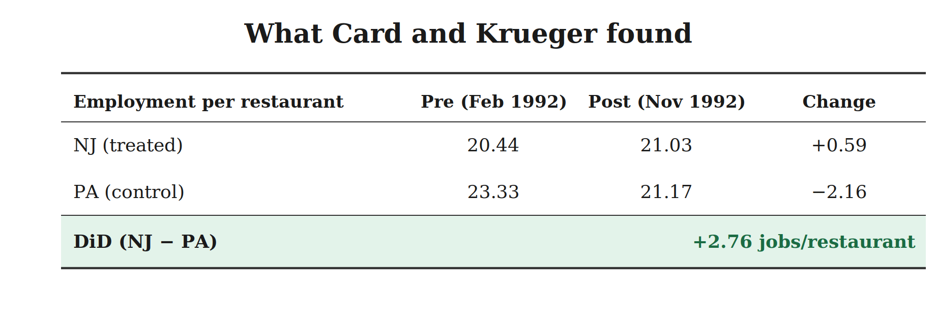
This is the standard 2x2. I’ll let the treatment be college. And the treatment group will be college educated workers, and the control group will be high school (only) educated workers. And the outcome, Y, will be their annual earnings. The classic 2x2 is:

\(δ^{2×2}=(Y_1,post−Y_1,pre)−(Y_0,post−Y_0,pre)\)

Let’s put it in a table so you can see it. You subtract left to right for each group to get their first difference. Then you go down and subtract those two first differences to get the diff-in-diff estimate.

It isn’t yet causal because it’s never causal until you have replaced observed outcomes with their corresponding potential outcomes. Once we do that, then we can see the causal term and the bias term. For now it’s just a simple calculation and nothing more.

I’ll show it to you now using the Card and Krueger results from their minimum wage paper. Be sure you always go “treatment first” when you do this. For first differences, it’s “after minus before” for the treated, then the control, then subtract the control first difference from the treatment group difference. See if you can find on here what the counterfactual trend is for New Jersey.

2. Group differences, the difference

Look closely at that table. Watch me now below. Instead of going left to right, we can go down and take group differences. Subtract the control group from the treatment group for both the before period and the after period. Then go left to right with that third subtraction and voila — you arrive at the same number. Why is that? Watch below.

\(δ^{2×2}=(Y_1,post−Y_0,post)−(Y_1,pre−Y_0,pre)\)

See, since the 2x2 is just a series of subtracted terms, you can move them around. And therefore because you can move them around, then the order doesn’t matter. The signs on them matter of course, but that’s what I mean by moving them around — you take the signs with you. And again here is the Card and Krueger representation of “group differences first”.

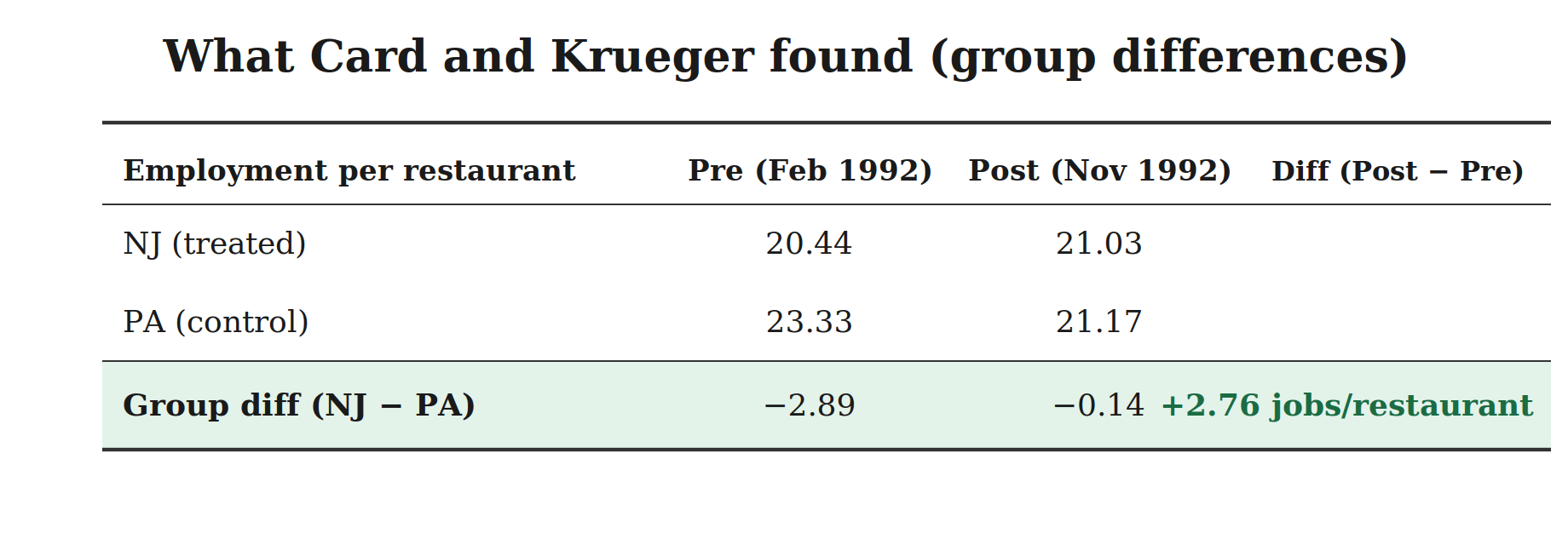
Notice that the 2x2 calculation is identical. Now see if you can figure out the “parallel group difference” is, as the parallel trends assumption remember is just another 2x2, but on Y(0) instead of Y, so it’s in here too. And remember — the “parallel difference” will have the exact same form as the 2x2 you calculated, so see if you can’t put what it is when we express it as group differences first.

---

Four Regressions

So there are two ways to write down the 2x2. But as most people don’t think of the diff-in-diff as a 2x2 in the first place — they typically see it as a regression, and a “two way fixed effects” regression at that — I think that doesn’t register as that big of a deal.

But did you know there’s four regressions that will calculate that exact diff-in-diff number? I mean by that that you can estimate the 2x2 using four different OLS regression specifications. Let me show you them.

1. Saturated regression (in dummies)

The first specification is simple. You create a treatment dummy equaling one for everyone in the treatment group combined and equaling zero for everyone in the control group combined. So this isn’t panel fixed effects. You also create a dummy for the post treatment period. And then this is the regression specification:

\(Y_{it} = \beta_0 + \beta_1 D_i + \beta_2\,\text{Post}_t + \delta\,(D_i \times \text{Post}_t) + \varepsilon_{it}\)

The coefficient on the delta is numerically identical to both of the manual four averages and three subtractions. We did. Both. Not just the first difference one — it’s also numerically identical to the group differences one.

2. Twoway fixed effects regression

Now instead of a single treatment dummy, put in a dummy for everyone — unit fixed effects in other words. Then run this.

\(Y_{it} = \alpha_i + \lambda_t + \delta\,(D_i \times \text{Post}_t) + \varepsilon_{it}\)

where alpha and lambda are unit and time fixed effects, respectively. And again, the delta coefficient is numerically identical to both of the manual 2x2 calculations as well as the previous regression we wrote down.

3. First difference regression

Next go in steps. First take a first difference by subtracting the baseline outcome from every units equation so that you are left with a cross-section and your outcome is now “difference in outcomes”. Then regress that onto a treatment dummy (no interaction).

\(\Delta Y_i = \beta_0 + \delta\, D_i + \varepsilon_i\)

That’s numerically identical to both 2x2 manual calculations, and both of the previous regression specs as well, but notice it went into two steps. You take a first difference, then you regress the first difference on to a treatment dummy.

4. Group difference regression

Finally, take group differences (treatment minus control) so that you end with two group values equal to Delta Y_t. Then regress that onto a post dummy.

\(\Delta Y_t = \beta_0 + \delta\,\text{Post}_t + \varepsilon_t\)

And here is the last one. This one you do the “group difference first” (i.e., delete the mean outcome for the control from the treatment in the pre and post period). Collapse it to time, then regress that on to the post dummy.

So you see, it’s not exactly accurate imo to refer to diff-in-diff as regression because it’s actually four regression specs, and it’s two different manual calculations. I encourage you to run this code to convince yourself.

* name: equivalence.do
* author: scott cunningham
* description: OLS and Manual are the same
clear 
capture log close
use https://github.com/scunning1975/mixtape/raw/master/castle.dta, clear
xtset sid year
drop if effyear==2005 | effyear==2007 | effyear==2008 | effyear==2009
drop 	post
gen 	post = 0
replace post = 1 if year>=2006
gen 	treat = 0
replace treat = 1 if effyear==2006
keep if year==2006 | year==2005

* Manual unweighted 2x2
summarize l_homicide if treat==1 & post==1
gen y11 = `r(mean)'
summarize l_homicide if treat==1 & post==0
gen y10 = `r(mean)'
summarize l_homicide if treat==0 & post==1
gen y01 = `r(mean)'
summarize l_homicide if treat==0 & post==0
gen y00 = `r(mean)'
gen did = (y11 - y10) - (y01 - y00)
sum did

* Regression Example 1: OLS regression with interactions (interactioned OLS)
reg l_homicide post##treat, cluster(sid)

* Regression Example 2: Twoway fixed effects (state and year fixed effects)
xtreg l_homicide c.treat#c.post i.year, fe vce(cluster sid)

* Regression Example 3: Regress "long difference" onto treatment dummy
preserve
    keep sid year l_homicide treat police
    reshape wide l_homicide police, i(sid) j(year)
    gen diff = l_homicide2006 - l_homicide2005
    reg diff treat, vce(cluster sid)
restore

* Regression Example 4: Regress "group difference" onto post dummy
preserve
    collapse (mean) l_homicide, by(treat post)
    reshape wide l_homicide, i(post) j(treat)
    gen gdiff = l_homicide1 - l_homicide0   // treatment minus control, each period
    reg gdiff post
restore

And if you wanted the weighted version:

* Now calculate the same thing using population weights as below
*Manual unweighted 2x2
summarize l_homicide if treat==1 & post==1 [aw=popwt]
gen wy11 = `r(mean)'
summarize l_homicide if treat==1 & post==0 [aw=popwt]
gen wy10 = `r(mean)'
summarize l_homicide if treat==0 & post==1 [aw=popwt]
gen wy01 = `r(mean)'
summarize l_homicide if treat==0 & post==0 [aw=popwt]
gen wy00 = `r(mean)'
gen wdid = (wy11 - wy10) - (wy01 - wy00)
sum wdid

* Regression Example 1: OLS regression with interactions and population weights
reg l_homicide post##treat [aweight=popwt], cluster(sid) 

* Regression Example 2: Twoway fixed effects (state and year fixed effects)
xtreg l_homicide c.treat#c.post i.year [aw=popwt], fe vce(cluster sid)

* Regression Example 3: Regress "long difference" onto treatment dummy
preserve
    keep sid year l_homicide popwt treat blackm_15_24 whitem_15_24 blackm_25_44 whitem_25_44
    reshape wide l_homicide popwt blackm_15_24 whitem_15_24 blackm_25_44 whitem_25_44 , i(sid) j(year)
    gen diff = l_homicide2006 - l_homicide2005
    reg diff treat [aw=popwt2005], vce(cluster sid)
restore

* Regression Example 4: Regress "group difference" onto post dummy (weighted)
preserve
    collapse (mean) l_homicide [aw=popwt], by(treat post)
    reshape wide l_homicide, i(post) j(treat)
    gen gdiff = l_homicide1 - l_homicide0
    reg gdiff post
restore

capture log close
exit

---

Concluding remarks

So the next diff in diff post will pick up on this by examining the different biases of linear regressions controlling for covariates. But today was merely to show that I’ll be working with the 2x2, I’ll be working with regressions that estimate the 2x2, and while I could do it any number of ways, I’ll be using for simplicity the saturated regression (the first spec above), as that’ll be more familiar I think to people.

But you never know! My hunch is it’s a strong belief for some, particularly people closer in age to me, that diff-in-diff a synonym for regression, and a particular regression (usually TWFE), but as I show, diff-in-diff is a 2x2 that can be estimated with regressions — just not technically the same regression specification. Yet weirdly, while you write them down differently, they are numerically identical on the point estimate. (Inference I’ll leave for another day if that’s okay).