Illustrating the bias of TWFE in event studies

Pretty little horrible pictures!

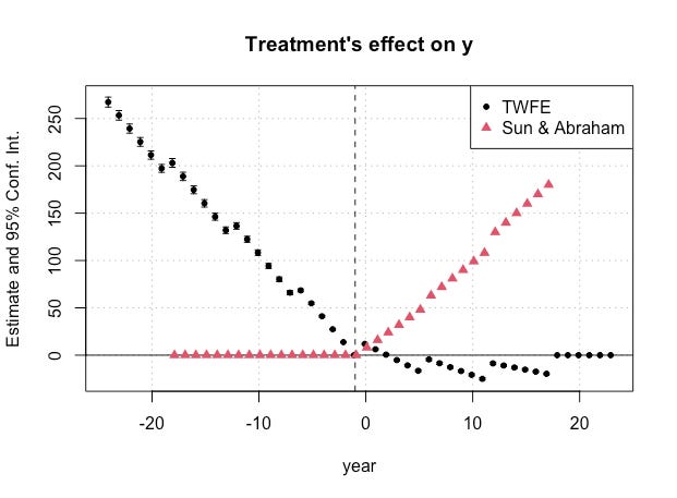
Introduction

The last few years in empirical micro and the broader quant social sciences has been a little stressful because of a series of papers by econometricians focused on the popular "difference-in-differences" design. Even Netflix uses that design. People may prefer A/B tests, but for some things, it's not feasible or realistic. Uber may not be able to run an A/B test on, for instance, a large new product because it would require flipping the switch across many geographic areas that could be very jarring for customers. So sometimes, these observational design approaches are valuable even if they aren't the slam dunk that you come to expect from an A/B test where physical randomization literally deletes from equations confounding selection bias terms.

But back to diff-in-diff. Starting in 2016, when a paper by Kirill Borusyak and Xavier Jaravel (then grad students) came out finding a lot of serious problems with a canonical specification of OLS models (called "twoway fixed effects", or TWFE), a slowly growing tidal wave started emerging on the horizon that eventually hit with around a half dozen or so high profile papers. Probably the most well known is one by Andrew Goodman-Bacon, then an assistant professor of economics at Vanderbilt, whose paper since 2018 has been cited about 1500 times. Contrast that with Alberto Abadie's 2005 semi-parametric difference-in-differences, probably the most famous of all the econometric papers on DiD, which is something like 2200 and is Abadie's fourth most cited paper after a couple of synth papers and you can get a sense of the impact of Bacon's paper. But there were others, too, several of which I’ve discussed on this substack.

I think when Goodman-Bacon's paper decomposing TWFE coefficients with differential timing into bias terms relating to dynamics in the treatment effects first came out, there was an initial hope that event studies would be preferable because maybe you skirt the issue by estimating dynamic coefficients directly. But Sun and Abraham (2020) in the Journal of Econometrics provided a careful decomposition of those population regression coefficients and in fact those are biased too, just for different reasons. Let’s dive into this closely by working with some simulated data. I call this data “baker” named after my friend Andrew Baker who had an old blog post written in R that generated these data. Here’s my baker.do code in Stata so you can follow along.

baker.do simulated data with extreme dynamics

This file contains bidirectional Unicode text that may be interpreted or compiled differently than what appears below. To review, open the file in an editor that reveals hidden Unicode characters. Learn more about bidirectional Unicode characters

Show hidden characters

	********************************************************************************
	* name: baker.do
	* author: scott cunningham (baylor) adapting andrew baker (stanford)
	* description: illustrate TWFE with differential timing and
	* heterogenous treatment effects over time
	* last updated: jan 5, 2022
	********************************************************************************
	clear
	capture log close
	set seed 20200403
	* 1,000 firms (25 per state), 40 states, 4 groups (250 per groups), 30 years
	* First create the states
	set obs 40
	gen state = _n
	* Finally generate 1000 firms. These are in each state. So 25 per state.
	expand 25
	bysort state: gen firms=runiform(0,5)
	label variable firms "Unique firm fixed effect per state"
	* Second create the years
	expand 30
	sort state
	bysort state firms: gen year = _n
	gen n=year
	replace year = 1980 if year==1
	replace year = 1981 if year==2
	replace year = 1982 if year==3
	replace year = 1983 if year==4
	replace year = 1984 if year==5
	replace year = 1985 if year==6
	replace year = 1986 if year==7
	replace year = 1987 if year==8
	replace year = 1988 if year==9
	replace year = 1989 if year==10
	replace year = 1990 if year==11
	replace year = 1991 if year==12
	replace year = 1992 if year==13
	replace year = 1993 if year==14
	replace year = 1994 if year==15
	replace year = 1995 if year==16
	replace year = 1996 if year==17
	replace year = 1997 if year==18
	replace year = 1998 if year==19
	replace year = 1999 if year==20
	replace year = 2000 if year==21
	replace year = 2001 if year==22
	replace year = 2002 if year==23
	replace year = 2003 if year==24
	replace year = 2004 if year==25
	replace year = 2005 if year==26
	replace year = 2006 if year==27
	replace year = 2007 if year==28
	replace year = 2008 if year==29
	replace year = 2009 if year==30
	egen id =group(state firms)
	* Add 250 firms treated every period with the treatment effect still 7 on average
	* Cohort years 1986, 1992, 1998, 2004
	su state, detail
	gen group=0
	replace group=1 if state<=`r(p25)'
	replace group=2 if state>`r(p25)' & state<=`r(p50)'
	replace group=3 if state>`r(p50)' & state<=`r(p75)'
	replace group=4 if state>`r(p75)' & `r(p75)'!=.
	gen treat_date = 0
	replace treat_date = 1986 if group==1
	replace treat_date = 1992 if group==2
	replace treat_date = 1998 if group==3
	replace treat_date = 2004 if group==4
	gen treat=0
	replace treat=1 if group==1 & year>=1986
	replace treat=1 if group==2 & year>=1992
	replace treat=1 if group==3 & year>=1998
	replace treat=1 if group==4 & year>=2004
	* Data generating process
	gen e = rnormal(0,(0.5)^2)
	gen te1 = rnormal(10,(0.2)^2)
	gen te2 = rnormal(8,(0.2)^2)
	gen te3 = rnormal(6,(0.2)^2)
	gen te4 = rnormal(4,(0.2)^2)
	gen te = .
	replace te = te1 if group == 1
	replace te = te2 if group == 2
	replace te = te3 if group == 3
	replace te = te4 if group == 4
	***********************************************************************************************************************
	* DGP: heterogeneous versus constant (but always across group heterogeneity)
	* Cumulative treatment effect is te x (year - t_g + 1) -- Dynamic treatment effects over time for each group.
	* How does (year - treat_date + 1) create dynamic ATT? Assume treat_date is 1992 and it is year 2000. Then, te=8 x (2000 - 1992 + 1) = 8 x (9) = 72. Group 2's TE rises from an 8 up to 72 in the t+8 year.
	***********************************************************************************************************************
	* Constant treatment effects. Notice, the treatment effect is constant.
	gen y2 = firms + n + te*treat + e // parallel trends IN EVERY PERIOD.
	* Data generating process with heterogeneity over time
	gen y = firms + n + treat*te*(year - treat_date + 1) + e
	* For group 1, the ATT in 1986 is 10
	* For group 1, the ATT in 1987 is 20
	* For group 1, the ATT in 1988 is 30 and so on
	* This is what we mean by "dynamic treatment effects" or "heterogeneity over time"
	** Estimation
	* Estimation using TWFE - constant treatment effects
	areg y2 i.year treat, a(id) robust
	* Estimation using TWFE - heterogenous treatment effects over time
	areg y i.year treat, a(id) robust

view raw baker.do hosted with ❤ by GitHub

These data were intentionally created to have severe dynamics so that I can illustrate some basic problems with the canonical static and dynamic twoway fixed effects (TWFE) model specifications. If you look at lines 81 to 90, you’ll see that I introduced some heterogeneity terms (10, 8, 6 and 4 corresponding to groups 1 to 4, respectively). I then use those terms in line 102 to generate a variable called y. Look closely at line 102. There are three important features I want to bring to your attention:

1. The data imposes parallel trends in every period because without treatment, Y=Y(0) the potential outcome without treatment, grows at a rate of n, which is simply linear. So the outcome satisfies parallel trends.

2. The data also satisfies a lesser known assumption in diff-in-diff designs called “no anticipation”. What is no anticipation you ask? It’s nothing more than saying that the treatment effects in some time period t-k are zero if there is no treatment in that same period. The treatment effects, in other words, will not happen as a result of forward looking agents anticipating a treatment in the future. That can be violated in our lives — I win the lottery, but don’t get paid for another six months, so I buy a house today. If anticipation is happening, it probably just means the treatment is a little different than you thought, and you have to redesign the study so that no anticipation holds. But putting that aside, note that I have “NA” because without treatment in the year of treatment (1986, 1992, 1998 and 2004 for groups 1-4 respectively), there is no treatment effect. That’s all we mean by no anticipation.

3. Last is heterogenous treatment effects. Notice — it’s not just that treatment effects grow over time. It’s that the treatment effect profile differs across groups. Group 1 grows at a rate of 10, group 2 at a rate of 8, and so on. This is heterogenous treatment effect profiles and is going to create a problem.

Now let’s look at the estimated regression coefficients on the event study leads and lags.

TWFE

First, let’s write down the model we are going to be estimating with TWFE.

This is basically the canonical event study model estimated with TWFE. The gamma term is supposed to be a vector of state fixed effects (but I’m horrible at that 1[.] notation so I just will use gamma s and assume you know it’s state fixed effects) and lambda is a vector of year dummies. The gamma tau terms are pre-treatment “leads” and delta tau are the post-treatment “lag” coefficients that we are going to estimate with TWFE. When we estimate this model on the baker dataset we get the following. I’ll embed the R code too so you can follow.

This file contains bidirectional Unicode text that may be interpreted or compiled differently than what appears below. To review, open the file in an editor that reveals hidden Unicode characters. Learn more about bidirectional Unicode characters

Show hidden characters

	# ------------------------------------------------------------------------------
	# name: baker_sa.R
	# author: scott cunningham (with massive help from grant mcdermott who basically
	# fixed all of it, so I think he's the author tbh)
	# description: implement SA on the baker dataset
	# last updated: february 20, 2022
	# ------------------------------------------------------------------------------
	# load libraries
	library(haven) # Read Stata .dta files
	library(fixest) # Sun & Abraham (and regular TWFE and high-dimensional FEs, etc., etc.)
	# load data
	baker = read_dta('https://github.com/scunning1975/mixtape/raw/master/baker.dta')
	baker$treated = baker$treat_date!=0 # create a treatment variable
	# NB: All units in this dataset are treated so above is kind of pointless
	# Naive TWFE Event Study (SEs clustered by state)
	res_naive = feols(y ~ i(time_til, treated, ref = -1) |
	id + year,
	baker, vcov = ~state)
	summary(res_naive)
	iplot(res_naive, main = "Naive TWFE")
	# Again, because all units are treated you could just as well have run the
	# following:
	feols(y ~ i(time_til, ref = -1) |
	id + year,
	baker, vcov = ~state) |>
	iplot()

view raw twfe.R hosted with ❤ by GitHub

Here's the picture you get when you run lines 28-31. It’s a plotting of the event study coefficients.

¹

Let’s look closely at this.

The “time_til” variable is simply a variable measuring how many years until a unit is treated. The fourth group is treated in 2004, for instance, so in 1980 it is 24 years until treated. But the 1986 group will only have 6 pre-treatment periods. Same kind of reasoning for the lags — only 1986 will have 23 post-treatment periods because the data ends in 2009, whereas the 2004 group will have 5 post-treatment periods.

Now recall what I said earlier: the variable, y, was generated so that 1) no anticipation held (so coefficients should be zero in the pre-treatment period) and 2) parallel trends held. So then why am I getting this insanity? And that’s where we go to Sophie Sun and Sarah Abraham’s excellent 2020 paper in Journal of Econometrics.

SA decomposition of leads and lags with TWFE

The problem with TWFE with differential timing is that to get unbiased estimates of those population regression coefficients in the dynamic event study model above, you need not just PT and NA — you also need homogeneous treatment effect profiles, but as my numbered bullets showed, we have heterogenous treatment effect profiles. There’s an excellent decomposition that they show which I’m going to post here that they call Proposition 1.

If you look at the slide labeled Proposition 1, you'll see what any of those leads or lags capture. It's the sum of three terms: numbers from the period you're measuring, numbers from other periods your not interested in. The second row are the numbers from other periods in your specification and the third row is from you omitted period, which for me will be -1.

²

Now what are these three rows exactly? Each row is a conceptually distinct number corresponding to the number you calculated with OLS for a given lead or lag. Let’s focus on the t-10 lead, though, as the pre-treatment leads are absolutely bonkers. Let me break down each line with another set of numbered bullets.

1. Top row. The t-10 lead is measuring information from comparing mean t-10 leads for a given cohort to an untreated cohort at some baseline of consideration. Notice the difference-in-differences calculation in it. I call this the “DiD equation”, but Bacon calls it the “2x2”. This is the good stuff because it actually goes with the lead we want to measure.

2. Middle row. But that same t-10 lead number also contains a second number which are DiD equations from the other leads and lags in that regression specification from earlier. In other words, if your model included not just t-10, but also t-9, t-8, …, t+1, t+2, then your t-10 number will contain not just information from that t-10 period — it will also contain information from the t+2 and so on relative time periods! Yikes. I really hope we can make that go to zero…

3. Bottom row. And finally, your t-10 number also contains information from your dropped period (here it’s the standard t-1 period).

Now look closely — those three rows aren’t just DiD equations. They’re weighted DiD equations. And each row’s weights sum to different numbers which I’ll just show here so you have it as a cheat sheet for later. The top row sums to 1; the middle row sums to 0; the third row sums to -1. Now let’s look what happens when we gradually introduce the three key identifying assumptions we need for TWFE to be unbiased: parallel trends (PT), no anticipation (NA) and homogeneous treatment profiles.

The first thing that happens when you assume parallel trends is that every DiD equation becomes a cohort specific average treatment effect on the treated group (i.e., the cohort in question), or the CATT. It’s the CATT, though, for that particular relative time period for that particular cohort summed and weighted.

Now let’s introduce NA and see what happens. What exactly is NA? All NA means is that CATT is zero for all pre-treatment periods. It’s called “no anticipation” because forward looking economic actors often make adjustments today in “anticipation” of treatments that happen tomorrow, but we need that not to happen for DiD designs, and if it’s violated, you have to solve that little conundrum somehow. That’s on you, and beyond the scope of this, but it’s something to think about. So, under PT and NA, we substitute CATT terms for every DiD equation, and we set all pre-treatment CATT terms to zero. That’s Proposition 3 below.

But then what about the fact that each cohort may have a different profile? That’s reflected in the fact that CATT can be different from one another. If we were to assume homogenous treatment profiles, though, all of the CATT terms would just become identical to one another and we’d probably just be better off calling it the ATT so that we don’t get confused.

Let’s look at a toy example to illustrate this, because I find that notation to be a huge pain for my brain.

³

I’m going to assume a balanced dataset of two pre-treatment periods (t-1, t-2) and two post-treatment periods (0, t+1) with two treated cohorts. But, to illustrate what happens in the event study regression with TWFE, I’m going to drop two periods: t-1 and t+1. Why omit a future period you may ask? Because I said so. We want to see why this is a problem and to do that we need to do it.

Remember our weighting? Own period weights sum to one (i.e., there’s a 1 coefficient on the first term). Included leads and lag weights sum to zero (notice 1/2 - 1/2 = 0). Excluded leads and lags weights sum to negative one (notice 1/2 - 1 - 1/2 = -1). So if we assume PT, we get causal terms. If we assume NA, then for our t-2 lead, the own period is zero (NA does that), and the last two terms are also since both are from the period we dropped, t-1. And under homogenous treatment effects, group 1’s CATT in period 0 equals group 2’s CATT in period 0.

But, then notice — that fourth term didn’t drop out. What is it? It’s the omitted period, t+1, CATT weighted by the remaining non-canceled out weight of 1/2. And thus our TWFE regression estimate on the t-2 lead is biased by 1/2 CATT for group 1 in the t+1 period.

Now let’s go back to our TWFE plots from above. I’ll repost it here too. Why are the t-k leads non-zero? Well, we imposed PT and NA which means all we have left are the second row bias terms and they’re not canceling out even though the weights sum to zero because the weights are describing CATTs that differ from one another mechanically due to the DGP chosen. That’s why they’re non-zero — they’re contaminated by the other periods and they decline because the means pull down the higher numbers as capture the smaller treatment effects.

SA Model

Sun and Abraham propose a simple fix to this. Since the problem of heterogeneity is caused by TWFE using the “already treated” as controls in those DiD equations, trick TWFE to not use them. This kind of subsetting of the data is not uncommon in causal inference. While OLS loves any and all variation it can find, causal inference is more cautious wanting only variation that captures adequate imputations treated group counterfactuals. So limiting who that can be is key to all of causal inference — even in the RCT itself (i.e., the controls are adequate representations of the counterfactuals under the independence assumption of physical randomization). The name of the SA estimator is called the interaction weighted estimator and all that it is is an estimate of the leads and lags using untreated controls weighted by an estimated share of units in a cohort. As the weights are consistent, and the leads are consistently estimated, then the interaction weighted estimator is too. They show that this estimator is asymptotically normal and derive its asymptotic variance.

Okay, so now let’s go back to our baker dataset and implement this estimator. The comparison group for SA’s interaction weighted estimator will be 1) any never-treated groups (we have none of those in baker dataset) and 2) the last cohort treated (which for us is the fourth group). To force SA to use only that last cohort as a control, we have to trick R by dropping all periods when everyone is treated. Here’s the R code for that (thanks to Grant McDermott at Oregon for helping me on this).

This file contains bidirectional Unicode text that may be interpreted or compiled differently than what appears below. To review, open the file in an editor that reveals hidden Unicode characters. Learn more about bidirectional Unicode characters

Show hidden characters

	# Sun and Abraham (SA20)
	unique(baker$treat_date)
	# This time, our SA implementation is a little different because we don't have a
	# "never treated" group. (Everyone get's treated eventually.) So, we'll use our
	# last treated cohort (i.e. 2004) as the control group. In practice this means
	# that we have to subset our data by dropping all observations after this final
	# treatment year. You could create a new dataset, but here we'll just use the
	# `subset` argument to drop these observations on the fly.
	res_cohort = feols(y ~ sunab(treat_date, year) | id + year,
	baker, subset = ~year<2004, ## NB: subset!
	vcov = ~state)
	summary(res_cohort)
	iplot(res_cohort, ref.line = -1, main = "Sun & Abraham")
	# Can also use iplot to plot them together
	iplot(list(res_naive, res_cohort), ref.line = -1,
	main = "Treatment's effect on y")
	legend("topright", col = c(1, 2), pch = c(20, 17),
	legend = c("TWFE", "Sun & Abraham"))

view raw sa.R hosted with ❤ by GitHub

The figure that this creates is great, because it puts the TWFE on the same figure as SA. And when you see them side by side, you can probably sense the problem — the descending plots for TWFE are the mirror image of the real ascending CATTs we identify with SA in the post-treatment period. Why? Because the descending plots are measuring them and the furthest lags are the furthest estimated leads in TWFE. The weird jagged declines you see with TWFE on the right are just the continual descending plots as groups graduate and leave the sample (first the 1998 group, then the 1992 group, and finally the 1986 group) as those do not have the entirety of that spectrum of lags.

Conclusion

The three core assumptions you need for TWFE to be a consistent estimate of population regression coefficients in a dynamic event study specification like we used above are 1) parallel trends, 2) no anticipation and 3) homogeneous treatment effect profiles. You need all three, not just the first two. And as units are often self selecting into treatment based on returns, it’s not surprising to expect that these profiles could differ. Such heterogeneities are practically guaranteed to occur when one considers the nature of rational agents reasoning about choices and expected gains.

Given the event study is such a crucial piece of technology for estimating casual effects with a DiD design, it would have been a bummer if Sun and Abraham diagnosed as terminally ill without giving us a cure, but like many others in this area, they didn’t. They gave us a simple fix that actually allowed us to continue to use TWFE. You just subset the data by only using the last cohort and the never treated units as controls, and then weight the coefficients by the shares that can be consistently estimated.

I want to leave you with one thing. At a conference I once attended, Father Don Rubin, one of our patron saints in design based causal inference, he said that with randomization we have confidence because “we know how the science works”. What science? When treatments are assigned independently of potential outcomes, then mean potential outcomes are equal across treatment and control which allows us to write down credible equations that delete selection bias in simple contrasts.

Well, difference-in-differences doesn’t use independence for identification. It uses parallel trends, and unlike randomization, there is no analog of a “science” to give us confidence. In its place, we use a variety of ad hoc statistical tests to give us assurances that while we cannot directly observe that Y(0) would have evolved similarly for all our treatment groups to the controls, we at least feel decent about it. And the most important piece of technology, as I said, for that is the event study. We don’t merely estimate event studies to better understand dynamics; we also do it because placebo estimation is a crucial tool we use in design based causal inference to check whether our identifying assumptions hold. We do it with RDD too to evaluate smoothness by checking our models’ performance on exogenous covariates as well as with the McCrary density test. Sure, it’s not perfect, but without randomization, we make due because of the importance of the questions we are engaged in.

1. Ignore that you can’t see the confidence intervals — they’re there, but the data has almost no noise so OLS is very precise. I do this only for illustrative purposes because I don’t want to clutter the picture with more unnecessary information.

2. I won't be dropping two leads but note SA and others recommend that or you end up with a kind of multicollinearity problem under differential timing. But note, TWFE cannot identify those coefficients with differential timing unless you drop two terms, not just one. Borusyak, Jaravel and Speiss (2021) suggest using theory to guide that decision, but oftentimes applied researchers do not have a handle on a theory that could help them, so use your best judgment.

3. I got this from Sun and Abraham itself. Like I said, it’s a fantastic paper.