Matrix Completion: Part 2

Performances with a simple parallel trends violation

Advertisement

Before we get into the simulation, can’t help but do a plug for the upcoming workshops on causal inference and design by me and Peter Hull. Come one, come all. Learn causal inference and all your wildest dreams will come true. But seriously, come sign up. If you’re needing help, these are the workshops. Previous attendees have reported religious ecstasy and wept as they realized that time is a flat circle, and as they realized which parts of causal inference was the hard parts, and which ones were the easy parts.

Matrix Completion Part 2

Here is an image inspired by your substack on matrix completion with nuclear norm regularization (MCNN) and its comparison with difference-in-differences (DID) estimators. The image metaphorically represents the exploration of MCNN's strengths and limitations through simple simulations and analysis. It conveys a sense of unraveling complex data patterns, embodying the journey of discovery and understanding in the world of statistical analysis. The visualization aims to capture the intrigue and curiosity surrounding the unexpected similarities between MCNN and DID, leaving the viewer with a sense of surprise and revelation. — Dall-E 3

I am doing a new series on “matrix completion with nuclear norm regularization” or MCNN for short. The substacks are designed to help me deepen my understanding of the method’s strengths but primarily its limits, which I think is some of the more subtle parts of the paper. I won’t be explaining the paper in a traditional way; rather I will be running simple simulations, doing analysis on usually 2-3 estimators (MCNN being one of them, and various diff-in-diff estimators the other). And I’ll be trying to interpret the results as I compare them while also rereading the paper while interactions with the simulations. I’m going to do that again today but still sticking with a simple data generating process (DGP) because the simpler the DGP, the fewer the number of explanations there are for what I don’t understand.

I will continue to work constant treatment effects. The design is a simple 2x2 with no staggered adoption. An unknown treatment assignment mechanism was used, and there are no covariates. There is non random assignment which in light of a slate of new working papers documenting the absence of “negative weights” under random assignment (“design”), I could’ve started with random assignment. But random assignment is a rich man’s sport whereas I live on the wrong side of the tracks where our assignments are non-random. And if I have random assignment, I’m not really going to be using causal panel models in the first place. So I’d prefer not to bake into the DGP things which don’t have some bearing on my work.

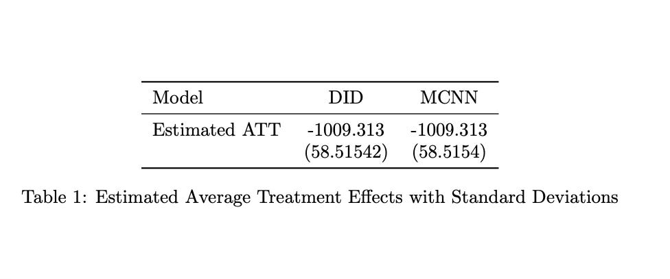
Yesterday’s post was interesting because the diff in diff results were numerically identical to the matrix completion with nuclear norm regularization (MCNN) results. Not similar in some “unbiased” sense the way propensity scores and a regression model might be very similar but not exactly the same. The results here were exactly the same. And I’ve been thinking about it and the main explanation I have is that it is because the fixed effects are not absorbed within the low rank matrix. They are estimated separately and then the regularization is performed to estimate the low rank matrix.

And yet, that procedure is numerically identical to a simple diff in diff model with NO year of unit fixed effects. Just a regression with a post treatment dummy, a single treatment group dummy — I mean a single dummy not many dummies — and its interaction. The coefficient on that interaction model is numerically identical to what I assumed was a very complex estimator that penalized a low rank matrix in a fixed effects regression. See here.

So there is definitely more under the hood if there is a situation where two seemingly very different specifications are in fact the same regression specification. I will have to keep plugging away and reading the paper again and again until I finally figure out why those two kinds of regressions are the same regression. But just so I’ve crossed this off, I’m going to do it one more time only today I will not have parallel trends. Other than that it’ll be the same as before — constant treatment effects, no staggering, no heteroskedasticity, balanced panel.

The data

My unit of observation is married women aged 20-40 average earnings at the city level. I don’t observe the workers wages; I observe a mean of all married women’s wages by city and I follow the same cities for 10 years.

There are 40 states, one of which is treated (“experimental”) and one of which is untreated (“non experimental”). The simulation is based on Gruber’s 1994 triple diff paper, but that’s just because I find it pedagogically helpful to stick with the same examples as long as I can so as to not clutter the mind with unnecessary details. The treatment is mandatory maternity benefits.

Baseline earnings was $40,000 in the non-experimental states and $80,000 in the experimental states (hence the non-random assignment I mentioned). But, after that, the two sets of states are different growth paths which automatically generates a violation of parallel trends. See here the code chunk.

* Annual wage growth for Y(0)
 quietly gen year_diff = year - 2010

* Setting trends for states and groups
 quietly gen state_trend     = 1000 if experimental == 1
 quietly replace state_trend = 1500 if experimental == 0

* Annual wage growth for Y(0) incorporating state and group trends
 quietly gen y0 = baseline + state_trend * year_diff

* Adding random error to Y(0)
 quietly gen error = rnormal(0, 1500)
 quietly replace y0 = y0 + error

So notice whereas yesterday Y(0) grew by $1000 per year for both experimental and non-experimental states, which gave us the parallel trends we used for estimation. Now, the experimental states grow by $1,000 per year, but the non-experimental states are playing “catch-up” growing faster at $1,500 per year. Thus when we use DiD, parallel trends will not hold, and DiD will be a biased estimate of the ATT, which equals -$1,000.

Estimation