Triple Differences Part 2

Case 1: Unbiased diff-in-diff and unbiased triple diff

From ChatGPT-4 after I requested an image illustrating triple differences. “Here's an abstract representation of the concept of triple differences in statistics and econometrics. The image is designed to symbolize the complexity and layered analysis involved in triple difference studies, with elements that suggest comparison, differentiation, and the intricate process of examining multiple groups across various time periods and conditions.”

I am thinking that this will be a simple substack, not some tome. And the reason it can’t be a tome is because I think all I really could pull off was this one simulation. The challenge for this one simulation is to help the reader understand it as an example of a historically common use of triple differences that I will just call “Unbiased diff-in-diff and unbiased triple diff”. And ironically, I am pretty sure this was Gruber’s original case, which makes it all the more awkward when I will say that triple differences is unnecessary in this situation, and you’d be better off doing what Miller, Johnson and Wherry did in their QJE and just present the “placebo DiD” alone.

My reasoning here is that if I show you this historical use case, even if it is one in which I argue triple differences was unnecessary in the first place as it doesn’t solve a problem, then a couple of things will happen. First, you can see my simulation. There’s some human capital I think with simulations. And if you can just start with a simple one, the reader gets used to my idiosyncratic way of writing code (if this can be called that). And I think there’s value to that to be honest because of what I want to do next.

What I want to do in part 3 is to present the “Case 2: Biased diff-in-diff and unbiased triple diff”. And I think if I can nail this really easy example, and you see the basics of all the triple diff stuff that in my opinion you need to know, like how to estimate it manually with “8 averages and 7 subtractions”, how to estimate it with a regression, how the data is structured, how the event study is estimated and how it is plotted, then I think you’ll be ready for the mind warped and poorly understood legitimate use case of triple diff which is for when you don’t have parallel trends.

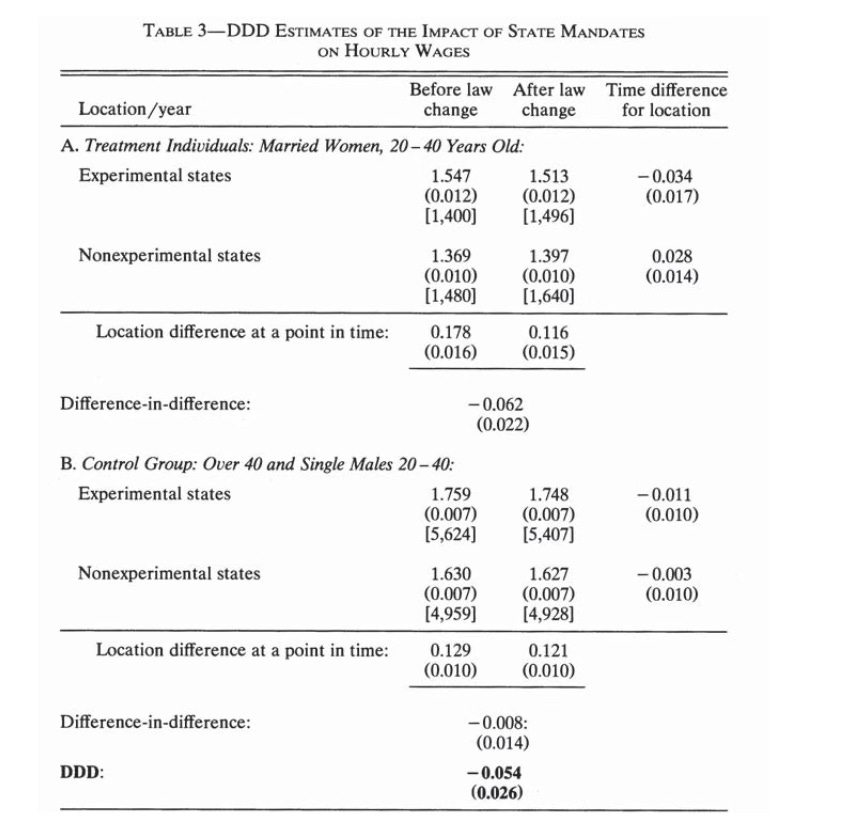
As promised yesterday, the first triple diff substack was free, but the rest you have to pay for. But I think you’ll like it because it’ll show you precisely what triple diff is from the ground up by generating the data using potential outcomes, giving you a known ATT, and then showing both DiD and triple diff point identify it. I’m not going to do a Monte Carlo, but maybe I’ll do that in the future. But just so you know what the code is trying to emulate, it’s inspired by Gruber’s 1994 AER, specifically this table.

These data are in log wages, and I chose to just use levels. But I’m going to have an ATT of -$5,000 which only affects married women ages 20-40 in this simulation. It’ll be the “maternity benefits mandate” idea, because I figure pedagogically, the more we can stick with the same stuff throughout this whole series, the more we can focus on the more subtler things and not have to reteach new frameworks each time. But that’s the table we are going shooting for, as well as a regression specification for it, and an event study for the triple Diff which I think has been a little rare. I should do a triple diff search on google scholar just to see how common this method even is.

Anyway, let’s get started. Below is the code.