Triple differences part 4: the simulation

This isn’t the last day of my triple differences series, but it’s getting there. I wanted to today to walk you through the material I covered yesterday but this time with a simulation. This will be a succinct, the point, substack. Here’s what you’ll find.

1. Biased diff-in-diff #1 (comparing states)

2. Biased diff-in-diff #2 (comparing groups)

3. Unbiased triple differences

And that’s it. I just think some people learn best when they see a simulation and if they see it laid out for them with equations. Not either/or but both/and. So this is the both/and.

Before I dive in, I’m going to plug the Mixtape Sessions workshops though. We are adding more slowly but wanted to get these four up for now. Okay, enough of that. Let’s simulate some data.

Data Generating Process

Let’s make some data now. If you want the entire thing in one place, just go to the bottom of the page because I have it there in one place for you. But I’m going to use code chunks like I did last week to provide commentary. This first part generates the potential outcomes, the realized outcomes and the treatment status.

We are going to stick with the original Gruber (1994) scenario in which we have two types of states. One state has mandatory maternity benefits (“experimental states”) and the others don’t (“non-experimental states”). Only people who are eligible for these benefits are pregnant women, but Gruber doesn’t have that data, so he uses instead “married women ages 20-40”.

clear
capture log close
set seed 20200403

* States, Groups, and Time Setup
set obs 40
gen state = _n

* Generate treatment groups
gen experimental = 0
replace experimental = 1 in 1/20

* 50 cities per state
expand 50
bysort state: gen city_no = _n
egen city = group(city_no state)
drop city_no

* Three groups per city: men (1), married women (2), and older women (3)
expand 3
bysort city state: gen worker = _n
egen id = group(worker city state)

* Time, 10 years
expand 10
sort state
bysort state city worker: gen year = _n

* Setting years
foreach y of numlist 1/10 {
    local year 2010 + `y' - 1
    replace year = `year' if year == `y'
}

* Define the after period (post-2015)
gen after = year >= 2015

* Baseline earnings in 2010 with different values for experimental and non-experimental states
gen 	baseline = 40000 if worker == 3  // Married women
replace baseline = 45000 if worker == 2  // Older women
replace baseline = 50000 if worker == 1  // Men

* Adjust baseline for experimental states
replace baseline = 1.5 * baseline if experimental == 1

* Annual wage growth for Y(0)
gen year_diff = year - 2010

* Setting trends for states and groups
gen state_trend = 1000 if experimental == 1
replace state_trend = 1500 if experimental == 0

gen group_trend = 500 if worker == 2
replace group_trend = 1000 if worker == 1 | worker == 3

* Annual wage growth for Y(0) incorporating state and group trends
gen y0 = baseline + state_trend * year_diff + group_trend * year_diff

* Adding random error to Y(0)
gen error = rnormal(0, 1500)
replace y0 = y0 + error

* Define Y(1) with an ATT of -$5000 for married women in experimental states post-2015
gen 	y1 = y0
replace y1 = y0 - 5000 if experimental == 1 & worker == 2 & after == 1

* Treatment effect
gen delta = y1-y0
su delta if after==1 & experimental ==1 & worker==2
gen att = `r(mean)'
su att


* Treatment indicator
gen 	treat = 0
replace treat = 1 if experimental == 1 & worker == 2 & after == 1

* Final earnings using switching equation
gen earnings = treat * y1 + (1 - treat) * y0

Different groups have different baseline earnings depending on which group they’re in and which state they’re in. I also have group trends and state trends which is going to create problems for parallel trends as you’ll see. The ATT is -$5,000.

Calculating 8 averages

I’m going to be running regressions, but I also like to calculate averages and take differences when teaching diff-in-diff. Not because anyone is ever going to calculate 8 averages and 7 subtractions in real life when estimating some ATT with triple differences, but because I want people to better understand what triple differences is, and why that specification I’ll show you does it. So let’s first calculate the 8 averages.

************************************************************************
* Calculating the 8 averages
************************************************************************

* 1. After, Married, Experimental
egen avg_wage_ame = mean(earnings) if after == 1 & experimental == 1 & worker == 2

* 2. Before, Married, Experimental
egen avg_wage_bme = mean(earnings) if after == 0 & experimental == 1 & worker == 2

* 3. After, Single Men and Older Women, Experimental
egen avg_wage_asoe = mean(earnings) if after == 1 & experimental == 1 & worker != 2

* 4. Before, Single Men and Older Women, Experimental
egen avg_wage_bsoe = mean(earnings) if after == 0 & experimental == 1 & worker != 2

* 5. After, Married, Non-Experimental
egen avg_wage_amn = mean(earnings) if after == 1 & experimental == 0 & worker == 2

* 6. Before, Married, Non-Experimental
egen avg_wage_bmn = mean(earnings) if after == 0 & experimental == 0 & worker == 2

* 7. After, Single Men and Older Women, Non-Experimental
egen avg_wage_ason = mean(earnings) if after == 1 & experimental == 0 & worker != 2

* 8. Before, Single Men and Older Women, Non-Experimental
egen avg_wage_bson = mean(earnings) if after == 0 & experimental == 0 & worker != 2

Now we have 8 averages: one for each before period and each after period for each group in each set of states. Let’s calculate our first (biased) difference-in-differences.

Biased diff-in-diff #1 — Comparing states

There are actually two ways we could go about estimating the ATT using diff-in-diff, but the one I’m going to do first is arguably the most common. Use two sets of states for one group (married women aged 20-40). We’ll call the experimental states “New Jersey” and the non-experimental states “Pennsylvania” in honor of Card and Krueger’s (1994) minimum wage paper which came out an issue later after Gruber’s 1994 paper.

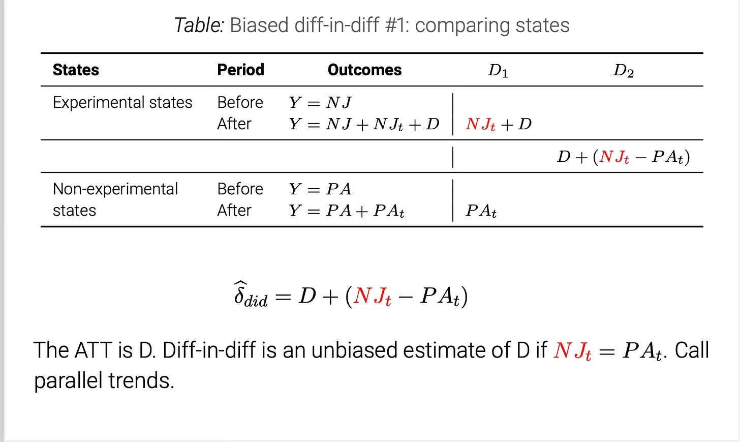
So, what exactly does NJ_t and PA_t mean? Let me show you with potential outcomes:

\(\begin{eqnarray*} NJ_t &=& E[Y^0_t - Y^0_{t-1}|D=NJ] \\ PA_t &=& E[Y^0_t - Y^0_{t-1}|D=PA] \end{eqnarray*}\)

I just use letters instead of the potential outcomes so that it can easily fit into the table. But the reason I put it in NJ_t in read is because that first term is counterfactual as the experimental states are treated in the post-period, meaning we observe Y(1), not Y(0). And if NJ_t=PA_t, then parallel trends holds, and that simple diff-in-diff will identify the ATT. But what if it doesn’t hold?

**************************************************************************** 
* Biased DiD Case 1: married women to married women but in different states
**************************************************************************** 

summarize avg_wage_ame, meanonly
local after_married_exp = r(mean)

summarize avg_wage_bme, meanonly
local before_married_exp = r(mean)

summarize avg_wage_amn, meanonly
local after_married_nonexp = r(mean)

summarize avg_wage_bmn, meanonly
local before_married_nonexp = r(mean)

* Calculate the DiD estimate
local DiD_case1 = (`after_married_exp' - `before_married_exp') - (`after_married_nonexp' - `before_married_nonexp')

* Display the result
display "Difference-in-Differences Estimate: " `DiD_case1'

If you run that entire code, you’ll get the following estimated diff-in-diff:

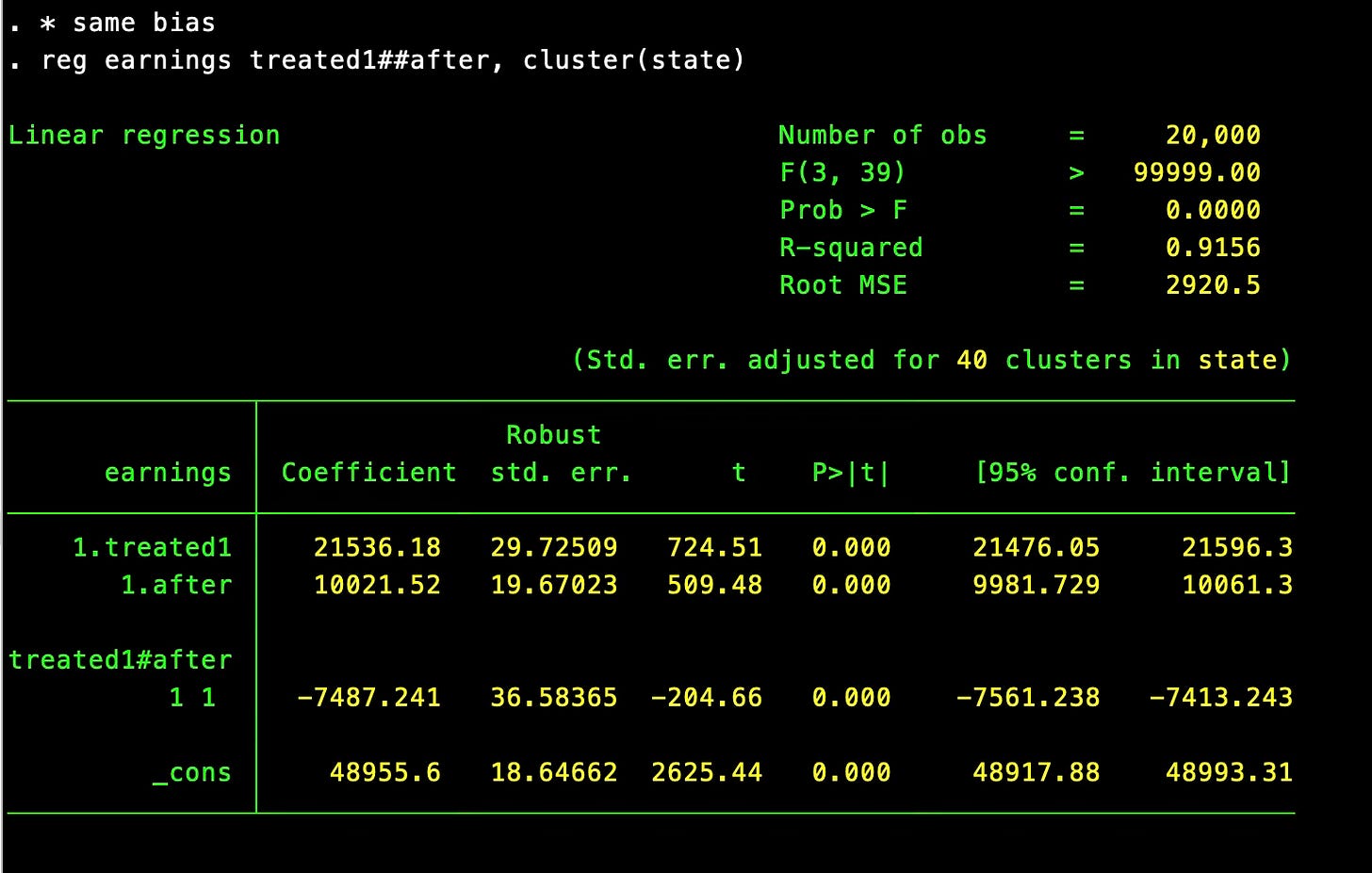
The ATT is -$5,000, and our DiD estimate is -$7,487.2422, which means NJ_t-PA_t = -2,487.2422. If you wanted to check for yourself, I encourage you to just calculate the non-parallel trends term directly yourself. (I’ll do it later in the second diff-in-diff). Now, we will run the regressions and plot the event study.

* Regression event study for biased DID. 
gen 	treated1=0
replace treated1=1 if experimental==1 & worker==2
replace treated1=. if worker~=2

* same bias
reg earnings treated1##after, cluster(state)

* Biased event study too
reg earnings treated1##ib2014.year, cluster(state)

coefplot, keep(1.treated1#*) omitted baselevels cirecast(rcap) ///
    rename(1.treated1#([0-9]+).year = \1, regex) at(_coef) ///
    yline(0, lp(solid)) xline(2014.5, lpattern(dash)) ///
    xlab(2010(1)2019)

The coefficient on the interaction of “treated1” and “after” is -$7,487.24 just like we found manually with our “four averages and three subtractions”. I’m not sure, actually, why it isn’t identical, but it’s probably something to do with rounding or how Stata stores different kinds of numbers.

Now let’s create our event study plot. We will use the user-created command “coefplot” created by Ben Jann.

* Biased event study too
reg earnings treated1##ib2014.year, cluster(state)

coefplot, keep(1.treated1#*) omitted baselevels cirecast(rcap) ///
    rename(1.treated1#([0-9]+).year = \1, regex) at(_coef) ///
    yline(0, lp(solid)) yline(-5000, lp(dot)) xline(2014.5, lpattern(dash)) ///
    xlab(2010(1)2019)

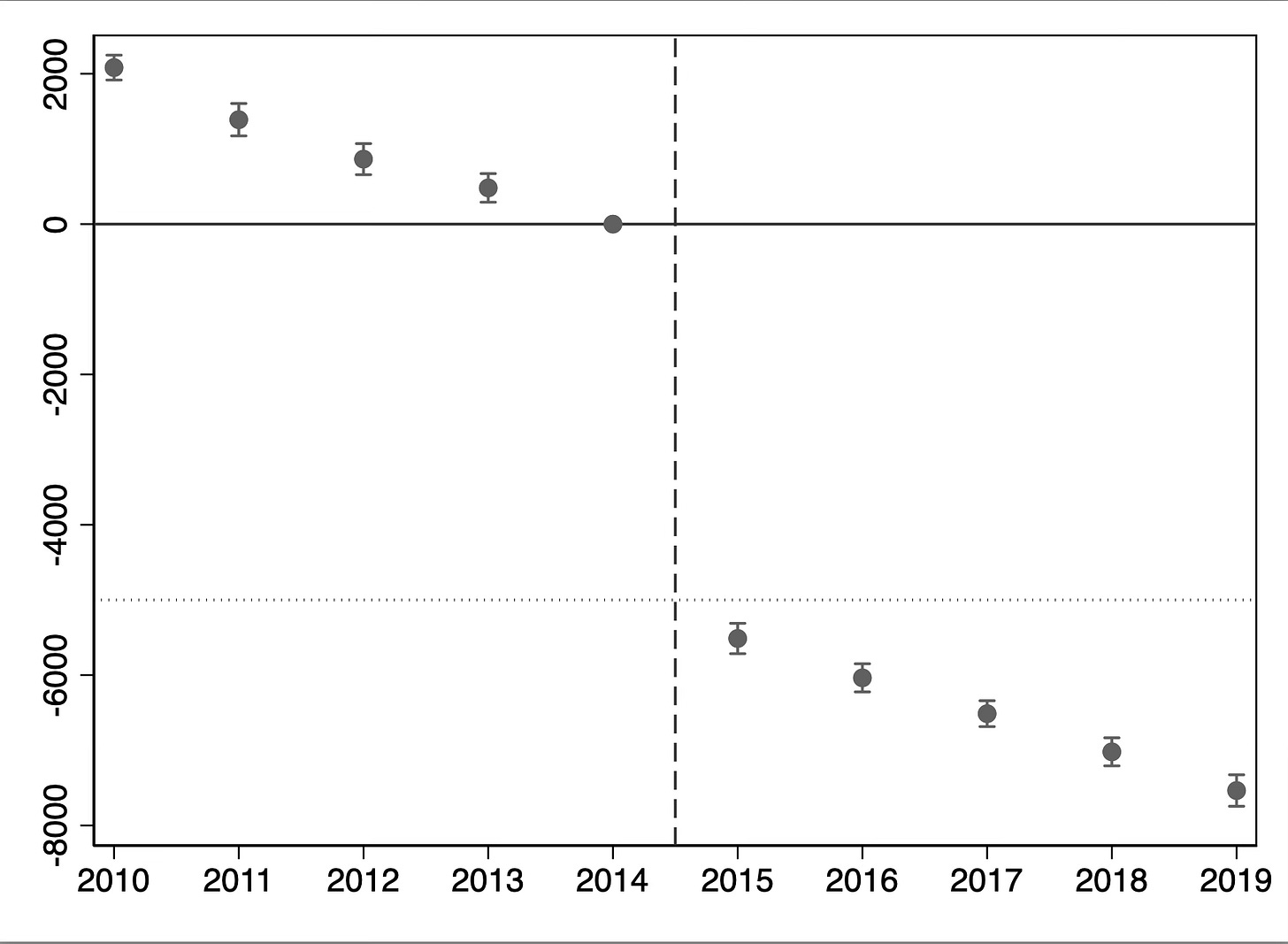
To save space, I’ll just show you the event study, but you can use that code to make event studies yourself too if you want. I put dots at -$5,000 so you could see that the ATT was actually -5,000 and instead we find a biased estimate. It’s actually a constant treatment effect, also, not dynamic. And we get a whiff of the problem when we look at the pre-trends; they are not parallel.

Let’s now look at a second diff-in-diff.