Claude Code 31: Apple-to-Apple Audit of Six Callaway and Sant'Anna packages

Six Packages, Same Estimator, Same Specifications, Same Dataset, Different Numbers!!! :(

This is part of a long-running series on Claude Code which began back in mid-December. You can find all of them here. My interest is consistently more on the end of “using Claude Code for practical empirical research” defined as the type of quantitative (mostly causality) research you see these days in the social sciences which focuses on datasets stored in spreadsheets, calculations using scripting programming languages (R, Stata, python) and econometric estimators. But I also write “Claude Code fan fiction” style essays, and then sometimes just like many wonder where we are going now with such radical things as AI Agents that appear to be shifting which cognitive activities and tasks humans have a comparative advantage in and which ones we do not.

For those who are new to the substack, I am the Ben H. Williams Professor of Economics at Baylor University, and currently on leave teaching statistics classes in the Government department at Harvard University. I live in Back Bay, and love it here — I particularly love the New England winters, the Patriots, the Celtics, the Red Sox, and New England as a region more generally. I enjoy writing about econometrics, causal inference, AI and personal stuff. I’m the author of a book called Causal Inference: The Mixtape (Yale University Press, 2021) as well as the author of a new book coming out this summer that is more or less a sequel/revision to it called Causal Inference: The Remix (also with Yale).

This substack is a labor of love. If you aren’t a paying subscriber, please consider becoming one! I think you’ll enjoy digging into the old archive. I also have a podcast called The Mixtape with Scott which is in its fifth season. This season is co-hosted with Caitlin Myers and we are doing a research project on the air using Claude Code to continue helping ourselves and others learn more about what is possible with AI agents for “practical empirical work”. Thanks again for joining — now read on to learn depressing facts about how six statistical packages for the identical econometric estimator with the identical specifications yields six extremely different answers to the same question and the same dataset. Sigh. I have three long videos belong. The first one shows me doing the experiment which I describe below, whereas the second and third one shows me reviewing the findings. Enjoy! And don’t forget to contemplate becoming a paying subscriber which is only $5/month! :)

Video 1: Setting up the Claude Codit Audit (52 minutes)

Slides 1-20 of the “beautiful deck” breakdown of CS analysis (52 minutes)

Slides 21-47 continued (43 minutes)

---

The Packages Didn’t Agree

I will tell this story in characteristic melodrama. If I were to try to explain this to my kids, they would think I am being a tad bit dramatic when I tell them the sky is falling because of the variation in estimates for the same estimator, same data, same covariates that I had found. But I would just say sticks and stones may break your fathers bones, but nothing hurts worse than when you make fun of me children so please stop and care about the things I care about.

But this substack isn’t about that. This substack is about the results of an experiment I did using Claude Code. Six packages, same estimator, same data, same covariates, with ATT estimates with as much as 50% of variation coming from which language-specific package you use, and coefficient estimates ranging from 0.0 to 2.38 on an important question (mental health hospital closures) and outcome (homicides).

One package said the treatment effect was roughly half a standard deviation. Another said it was more than double that.

---

Six packages implement one estimator

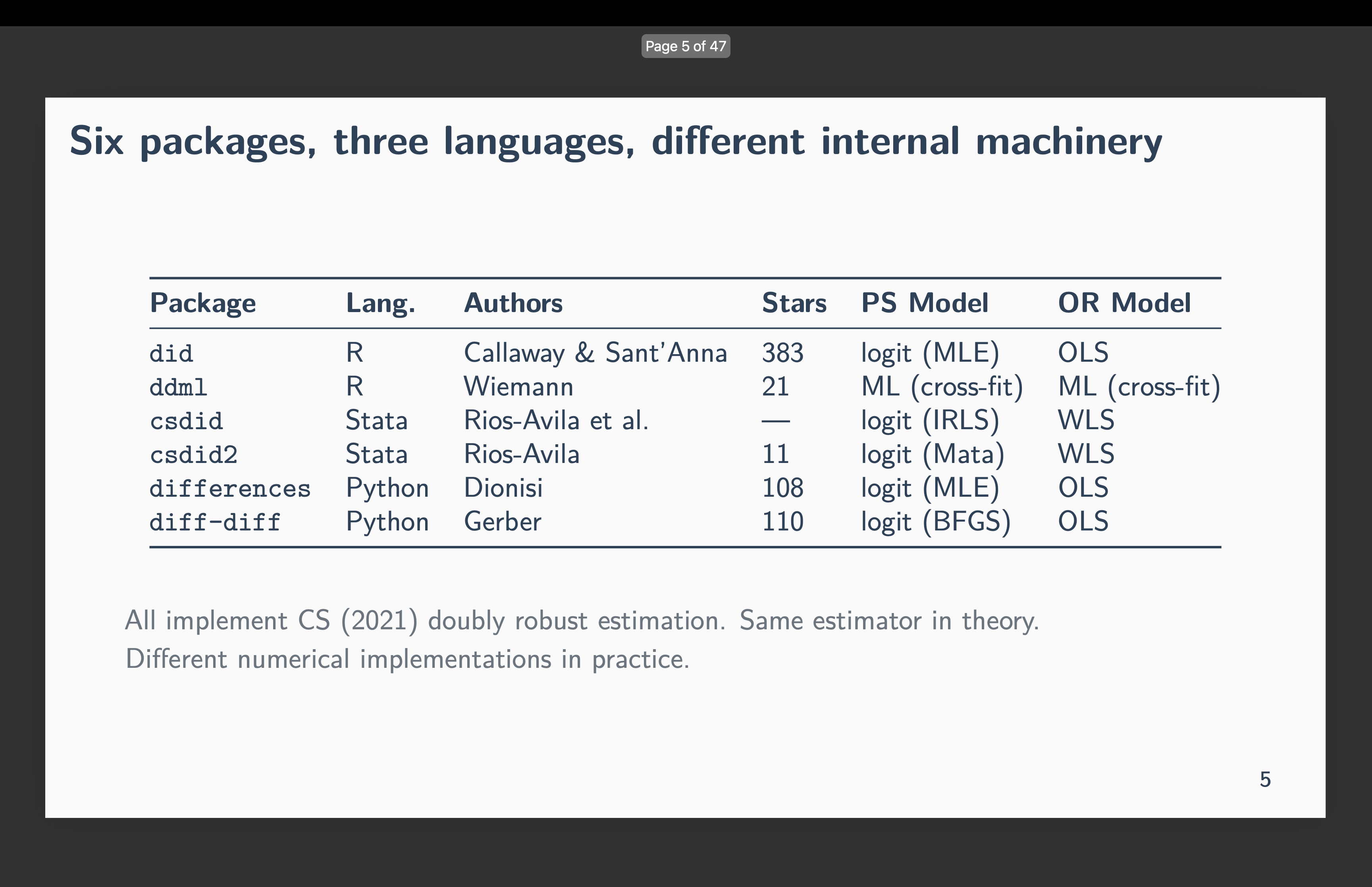
Callaway and Sant’Anna (2021) or CS has over 10,750 Google Scholar citations. Six independent teams built software to implement it:

• did (R) — Callaway and Sant’Anna themselves

• ddml (R) — Ahrens, Hansen, Schaffer, and Wiemann

• csdid (Stata) — Rios-Avila, Sant’Anna, and Callaway

• csdid2 (Stata) — Rios-Avila

• differences (Python) — Dionisi

• diff-diff (Python) — Gerber

My experiment was straightforward — have Claude Code wrote almost 100 scripts (16 specifications across all six packages in three programming languages simultaneously) to determine the “between” or “across-package” variation in estimates, as well as the within. I chose the same estimator (CS) with the exact 16 specifications so that I could figure out precisely what was driving the variation if it existed, as well as measure how large it is. But the idea is simple: CS is four averages and three subtractions with a propensity score and outcome regression.

None of that is random excluding the bootstrapped standard errors (which I do not investigate) and thus the only thing that can explain variation in estimated ATTs is package implementation of the propensity scores, the handling of near separation in that propensity score by the language-specific package, and any subtle issues like rounding. As it is not even common for economics articles to report which package and version they used of an estimator, let alone perform the kind of diagnostics I do here (i.e., 96 specifications across six languages to investigate the above issues), I think the findings are a bit worrisome.

But as I’ve written before, I think one of the real contributions that Claude Code and AI agents more generally can bring to the table is the role of the subagents to perform various types of, let’s call it, “code audit” on high value, time intensive, high stakes problems. And that is precisely what this is:

This is exactly the kind of “high value, time intensive, difficult, high stakes” work that AI agents should do. Writing identical specifications across R, Stata, and Python would ordinarily mean either being competent in multiple programming languages, packages in a language, econometrics, and good empirical practices (e.g., balance tables, histogram distributions of propensity scores, falsifications). A person with such skills is either usually not one of us, and probably not our coauthors, and if we know of someone like that, they are probably people with very high opportunity costs and aren’t going to loan us their expertise for a month or two of work that is ultimately just tedious coding work.

But Claude Code can, but also should, do this. And so part of my conclusion in this exercise is a simple policy recommendation for all empiricists: do this. Use Claude Code to perform extensive code audits. You can find my philosophy of it here at my repo “MixtapeTools” and my referee2 persona specifically. Just have Claude Code read it and explain the idea of referee2 which tries to simply replicate our entire pipelines in multiple languages to catch basic coding mistakes. But in today’s exercise, it was also to document that sometimes there is no coding mistake and yet the estimates from different packages may vary widely. But a code audit would’ve found that too.

---

The packages didn’t agree

So here is the gist. The data come from a staggered rollout of mental health centers across Brazilian municipalities, 2002-2016. I have 29 covariates covering demographics, economics, health infrastructure, and population trends. Sixteen specifications sample the space from zero covariates up through all 29. All variation is coming from covariates, both within a package (i.e., which covariates) but more importantly across packages. And that’s the headline — even for identical specifications, you can get variation in estimates and sometimes as much as anywhere from an ATT of zero to an ATT of 2.38. Even if you drop the zero, some specifications yielded estimates ranging from 0.45 additional homicides to 2.38 homicides (measured as a municipality population homicide rate).

A five fold difference in estimated effects of a mental health hospital changing in the homicide rate is not trivial.

Zero covariates. I know it is the covariates because with zero covariates, all five packages agreed to four decimal places: ATT around 0.31. The data are identical, the estimator is identical, the baseline works. And so this becomes one of my recommendations: always look at the baseline without covariates in your coding audit, not because you believe it is the correct estimator, but because it’s the simplest specification, and helps determine some basic facts before you go further.

One covariate. Then I added one covariate — poptotaltrend, a population trend variable — the estimates fanned out across estimators. For that single-covariate specification, the ATTs ranged from 0.45 (ddml) to 1.15 (csdid).¹ Add a few more covariates and the R package did started silently returning zeros. Though you would see the output that clearly indicates a problem, I think the fact that it is spitting out zeroes for the ATT (and NAs for the standard error) is more easily missed going forward if people are using AI agents outside of the R Studio environment. So I document it anyway and note that for those 9 out of 16 specifications, the ATT = 0.000, SE = NA.

But importantly — that does not happen for the others. So you have R’s did refusing to do the calculations (but which still had a zero ATT), but you have the others going forward. How is that possible exactly? Or maybe why is the better question.

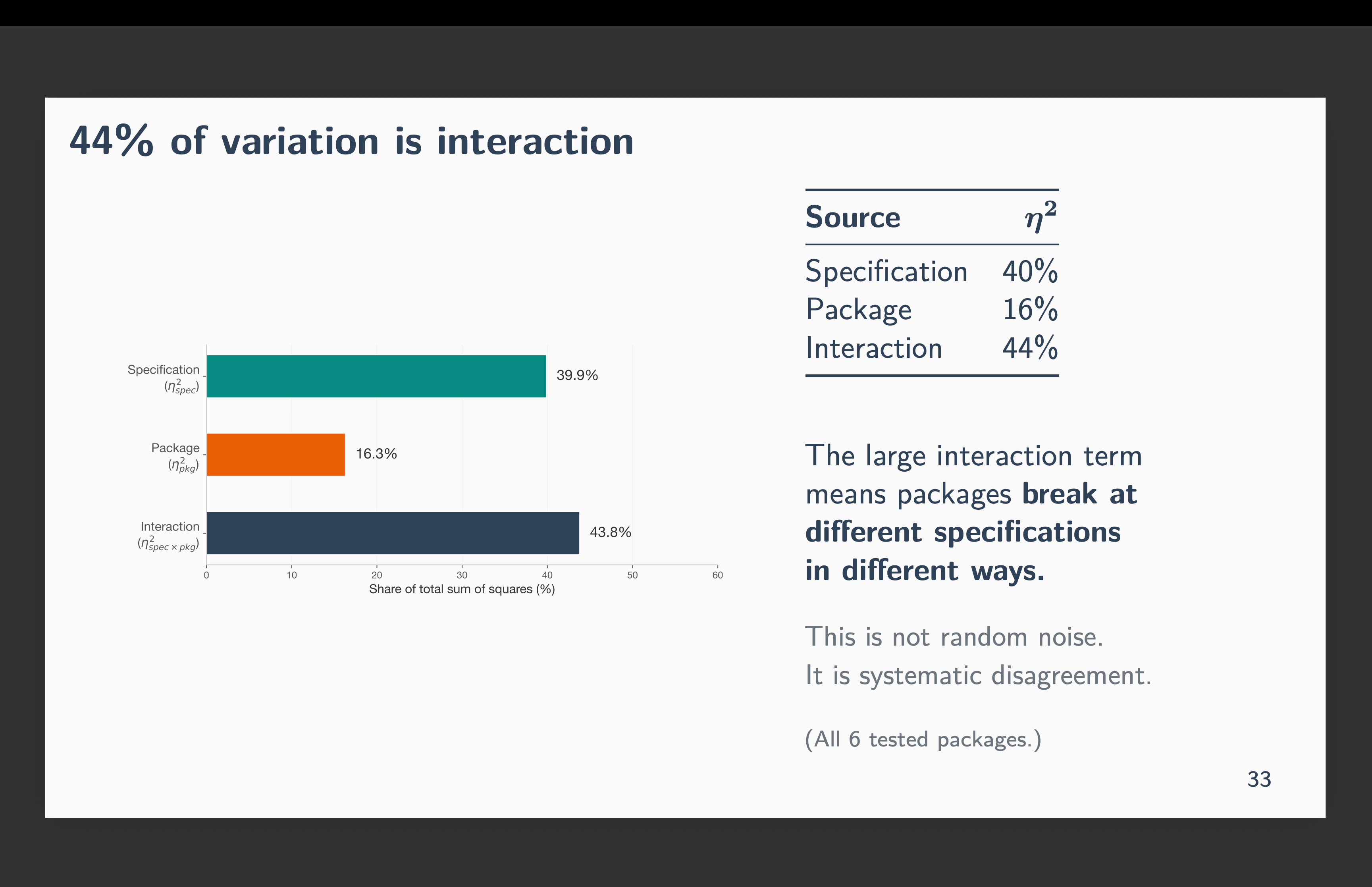
I asked Claude Code to calculate a two-way ANOVA decomposition of the variation in these estimates to try and unpack the story a bit more. Forty percent of the total variation in ATT estimates comes from specification choice — which covariates you include. Sixteen percent comes from package choice — which software you use, holding the specification fixed. And 44 percent is the interaction: packages breaking at different specifications in different ways. That interaction term is not noise. It is systematic disagreement.

The figure below shows the specification curve — one line per package, x-axis is the 16 specifications ordered by number of covariates. And each dot above the notches on the x-axis represent the simple ATT. So when there are vertical gaps, it means they disagree, and when they are on top of each other, they all agree. Note that at the baseline they’re stacked on top of each other. But when we include population trend, estimates fan out. By the time you hit three or four covariates, the lines are spread across a range wider than the estimate itself. It is at k=4 also that R’s did began spitting out zeros.

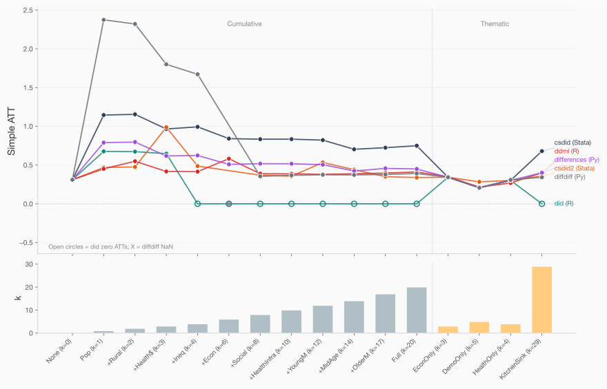
The gray lines specifications all include population trend as a covariate. The last one labeled “Kitchen Sink” includes all 29 covariates (including population trend). And the ones labeled “Econ only (k=3), DemoOnly (k=5) and healthOnly (k=4)” include 3, 5 and 4 covariates from those descriptions (but not population trend). Note that those three mostly agree — the discrepancy are largest when population trend was included.

---

The diagnosis is numerical, not econometric

The culprit is poptotaltrend. Why is that? Because it is equal to the population of the municipality multiplied by the year. That’s how the trend is modeled. But some municipalities are gigantic. For instance Rio has almost 7 million people. Whereas rural municipalities are not surprisingly much smaller. When multiplied by the year, you end up with the value being up to 10 billion.

So what? A number is a number, isn’t it? What’s so hard about a “big number” anyway?

Here is what Claude Code thinks is going on. He thinks the problem is coming not from the econometric estimator but from how each package is storing large numbers.

Computers store about 15-16 significant digits in a 64-bit floating point number. When two columns of your covariate matrix differ by a factor of 10 billion, the matrix inversion that sits inside every propensity score and every outcome regression cannot distinguish the small column from rounding error. The condition number of the design matrix — a measure of how much error gets amplified when you invert it — exceeds the threshold where computation becomes unreliable.

So that’s the first problem — it has to do simply with how a large number is getting stored and the implications of a large number with matrix inversion. But that is actually fixable, too. You can just divide a large number by another large number. And yet that is not the only problem even though that is a major part of the problem in the picture above.

---

The role of near-separation in the propensity score

The deeper issue is near-separation in the propensity score. With 29 covariates and some treatment cohorts as small as 47 municipalities against 4,000 controls, certain covariate combinations perfectly predict treatment assignment. The estimated propensity score hits zero or one for those units. The inverse probability weight — which is the propensity score divided by one minus the propensity score — goes to infinity. Common support fails.

Again, so what. Any explanation you give like that is generic. It should be failing for all the packages, right? This is where there is some things under the hood that most people never see. This is the hidden first stage that most applied researchers never see.

As a quick aside, I think one of the casualties of economics ignoring propensity scores for several decades is that we don’t know the basic diagnostics with respect to propensity score — like checking for common support with histograms or in this case checking for near separation, or even what that means. And you’d be fine if you never ran propensity score analysis in principles — except that propensity scores are under the hood in CS, and in marginal treatment effects with instrumental variables. And those methodologies are popular, and since they have propensity scores inside them, we are unknowingly venturing into waters where we maybe have deep knowledge about diff-in-diff, and even CS potentially, but shallow to no knowledge about propensity score, and thus really don’t realize what to check, or even to check. Particularly when these propensity scores are not being displayed within the larger package output itself.

Not to mention that many people write Callaway and Sant’Anna as a regression equation and move on. So even then there’s a fair amount of distance people are having in practice with the propensity score, even for a popular estimator like CS. Which is why I think it is vital that we learn it — even if you are going to just use diff-in-diff. Because if you use diff-in-diff, you will be using propensity scores at some point, but you may not realize it. And if a paper writes down a regression equation and says they estimate it with CS, they almost certainly don’t realize it otherwise there would be a propensity score in the equation.

So underneath, every doubly robust estimate requires both a propensity score model and an outcome regression. When you have 29 covariates, you have 536,870,911 possible covariate subsets — that’s 2 to the 29 minus 1. This is called “the curse of dimensionality”. And you can hit that curse far, far earlier than the kitchen sink regression. And when you have k>n (i.e., more dimensions than observations), you will have more parameters than units, and so you cannot even estimate the model.

Which is fine when all packages tell you this or do the same thing, but they do not all do that. And even if you can see it from R Studio, if we are moving towards automated CLI pipelines, we may not see whatever the packages are spitting out anyway.

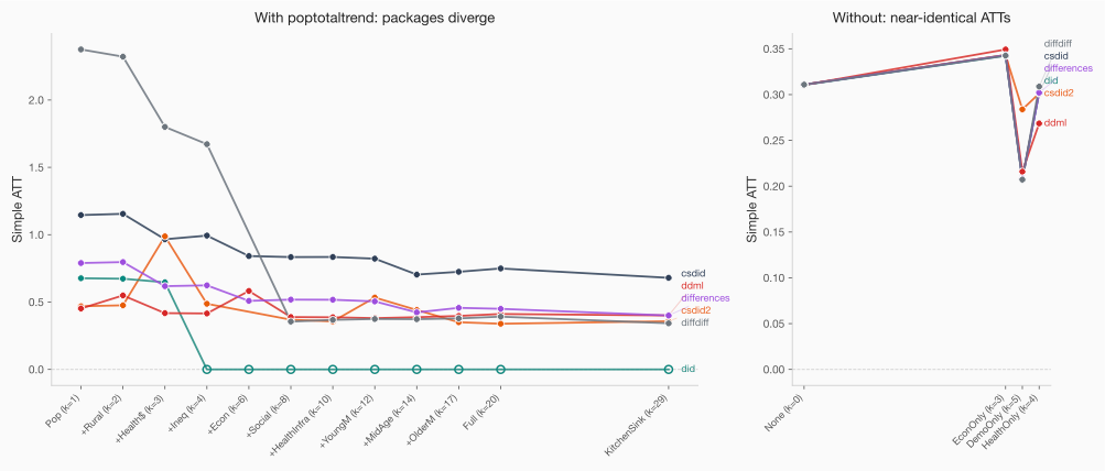
Remove poptotaltrend from the covariate set and all five packages agree to within 0.007. The between-package gap drops from over 0.57 to under 0.08. The left-hand side shows the divergence with poptotaltrend; the right-hand side below shows without. Notice how dropping gets us closely to near identical ATT estimates.

And here’s the thing that keeps me up: this isn’t really about difference-in-differences. A simple logistic regression would have the same near-separation problem with the same covariates. This goes beyond Callaway and Sant’Anna. Any estimator that depends on a propensity score is exposed and that is because the packages all differ with respect to the optimizer used (more below on that).

---

Z-scoring solves one problem but not the other

If the “big number” problem is because it’s a big number, then let’s address that by making all numbers in the same scale. Let’s standardize our covariates and try again.

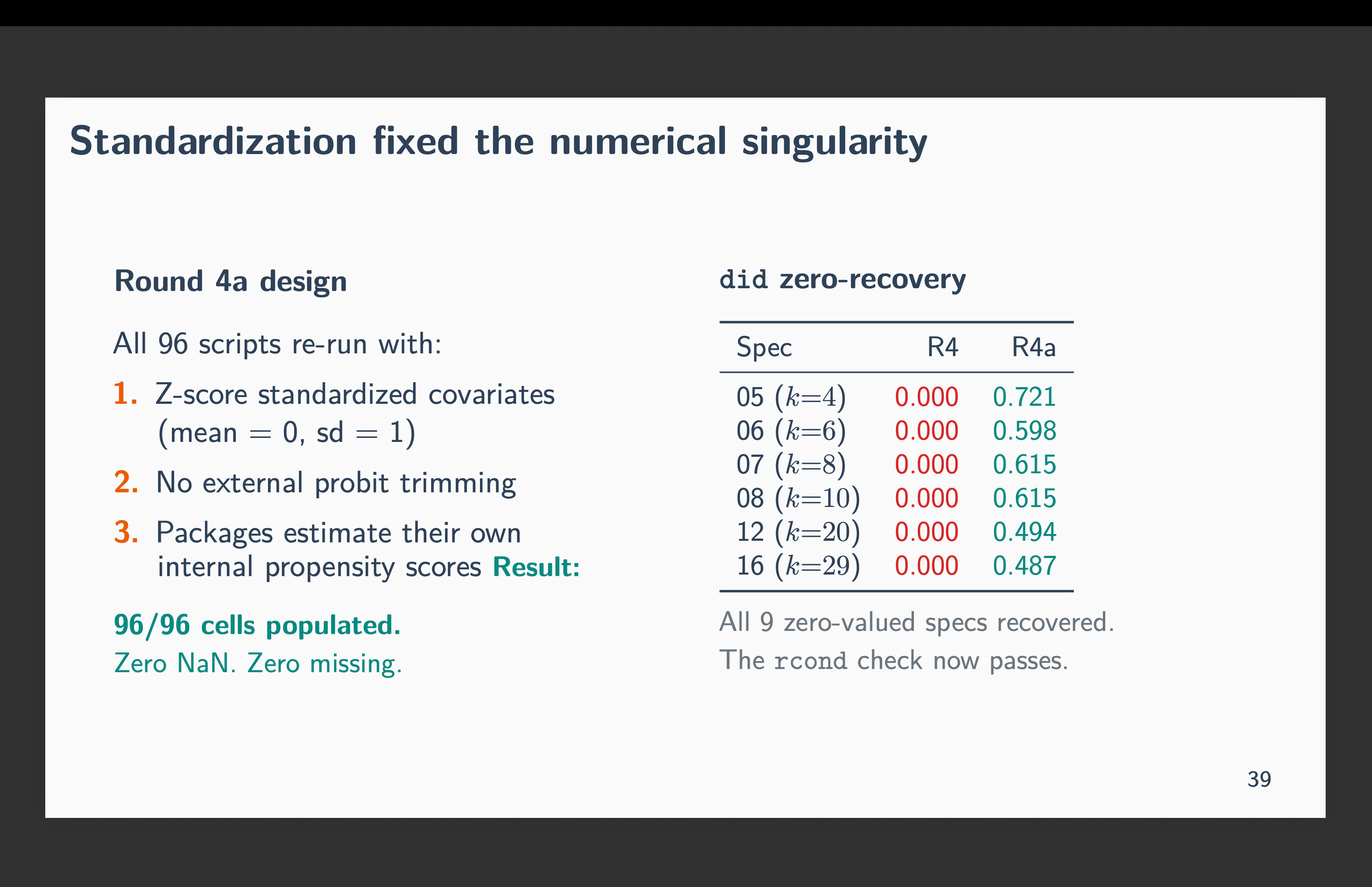
So, I re-ran all 96 scripts with z-score standardized covariates through demeaning and scaling by the standard deviation. This gives us a mean zero and standard deviation one. In other words, turn each covariate into a z-score. When I did this, the condition number dropped to roughly 1. Every zero recovered. All 96 cells produced real ATT estimates. The numerical problem was gone. For instance, no longer does R’s did refuse to calculate anything — at least now we are getting non-zero values for all 96 calculations.

And yet, csdid still estimated ATTs roughly twice as large as the other packages. The fan narrowed but didn’t close. You can see these new results here.

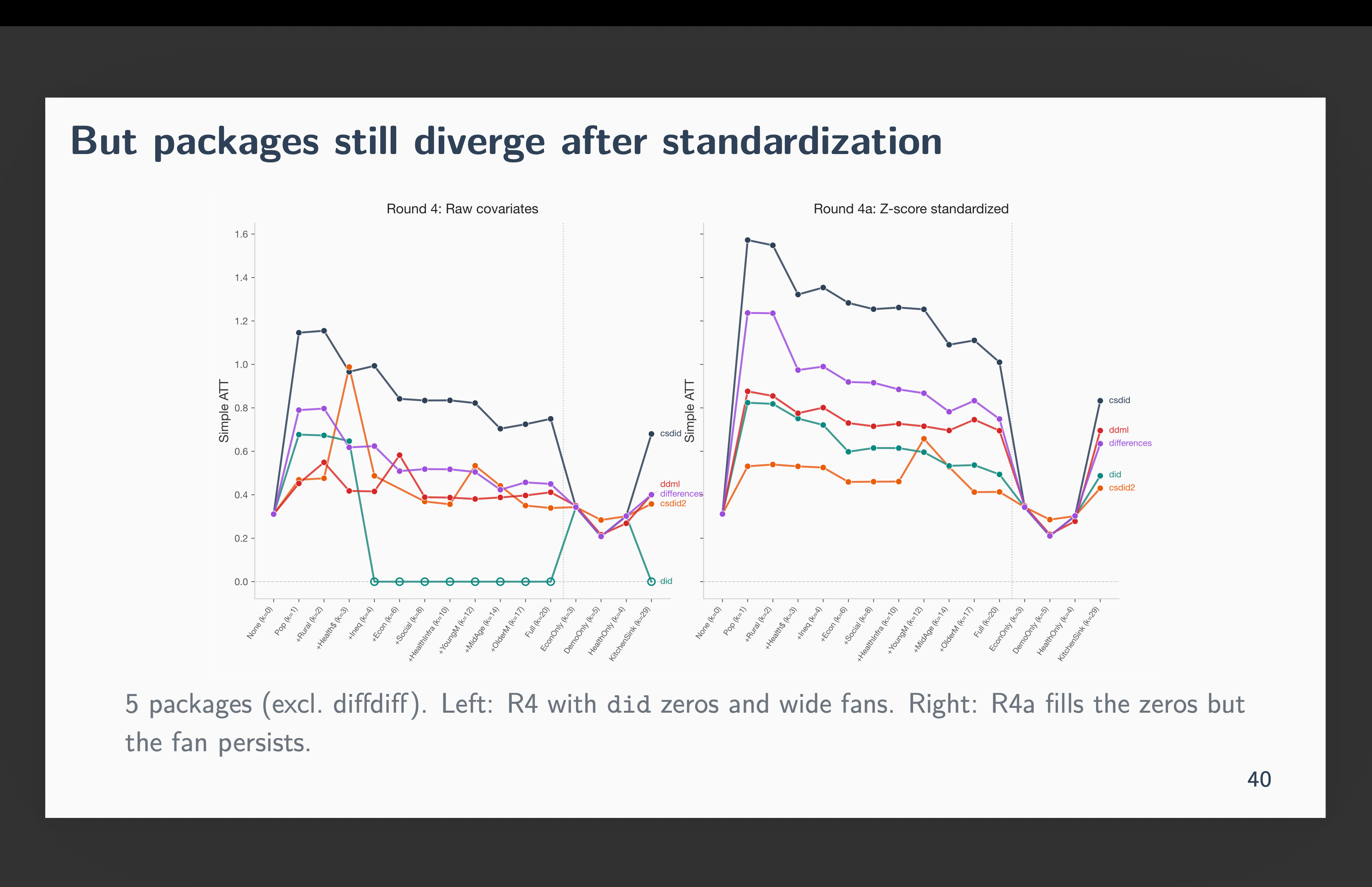
Why is this happening if we now no longer have “big numbers”? Because of “near-separation” from the propensity score stage creating outliers. Near-separation is about outlier structure, not scale. Z-scoring preserves outliers — a municipality that’s 8 standard deviations from the mean is still 8 standard deviations from the mean. It’s just no longer 10 billion compared to 0.4 as the mean of each covariate is zero and its standard deviation is 1.

The problem is that each package uses a different logit optimizer to estimate the propensity score, and each optimizer handles near-separation differently. did uses MLE logit. csdid uses inverse probability tilting, which finds weights that exactly balance covariates between treated and controls — and when near-separation is present, it assigns extreme weights to achieve that balance. Different propensity scores, different ATTs.

So, to summarize — standardization of covariates into z-scores fixed the computer’s problem, but not the statistical problem. The statistical problem remains even with z-scores as that has to do with outlier structure and perfect prediction of the propensity scores therefore in enough cases.

---

This is a new hidden action

This isn’t about researcher discretion — every package received the same specification. It also isn’t about parallel trends — we never got that far. Heck, it’s really not even about CS. This is actually about the way that each package brings in the propensity score and how it deals with numbers, and how it handles failures. In one case, failure caused for instance the estimator to just drop all of the covariates despite being told to use them and revert back to the “no covariate” case. And that is decidedly not clear whatsoever.

This is implementation variation buried in source code. Package choice is a substantive decision that determines whether your ATT is 0.00, 0.45, 1.15, or 2.38, and no journal requires you to report which package you used, and “robustness” is rarely if never going to involve checking a different language’s different package, or even different versions of the same package.

I’ve been calling it “orthogonal language hallucination errors” — the idea that if you run the same specification in three languages and they don’t agree, something is wrong, and the errors across languages are unlikely to be correlated. When Claude Code writes six pipelines and two of them disagree with the other four, that’s informative. It’s a code audit that would have been prohibitively expensive to do by hand.

Between-package variation is a previously undocumented source of publication bias. Not the kind where researchers choose specifications to get significance — the kind where the software silently produces different answers and nobody checks.

---

Where this leaves us

So I would not be a good economist if I did not finish a talk with “policy recommendations”. Here are four policy recommendations therefore.

1. First, report the package and version. Even after standardization, package choice produces roughly 2x different estimates.

2. Second, standardize your covariates before estimation. It eliminates numerical singularity and reduces interaction variance by a third.

3. Third, run a zero-covariate baseline.

4. Fourth, Confirm packages agree unconditionally before you start adding covariates and watching the results diverge — not because you think the proper specification is “no covariates” but because it’s the simplest case and you can rule out ways the packages are handling covariate cases.

But then here is a fifth point. The fifth point, and the broader point, is that this kind of cross-package, cross-language audit is exactly what Claude Code should be used for. Why? Because this is a task that is time-intensive, high-value, and brutally easy to get wrong. But just one mismatched diagnostic across languages invalidates the entire comparison, even something as simple as sample size values differing across specifications, would flag it. This is both easy and not easy — but it is not the work humans should be doing by hand given how easy it would be to even get that much wrong.

You can skip around the videos. The last two is me going over the “beautiful deck” that Claude Code made for me, and that deck is posted on my website.

If you find this kind of work useful — using Claude Code for practical research, not influencer content — I’d appreciate your considering a paid subscription. This is a labor of love, and there’s more to dig into. Not just Callaway and Sant’Anna. Every estimator that depends on a propensity score. Every package that inverts a matrix without telling you the condition number.

The TL;DR though is that tthe packages didn’t agree. And none of them told you. And sometimes mental health deinstitutionalization had no effect and sometimes it had 2.4 more homicides per capita. And it’s not because of “robustness” stuff — they should be identical and they weren’t.

1. I am omitting the python diff-diff discussion for the most part, though you can find it in the deck and videos. Mainly because it’s the newest, and still having some bugs worked out.